Comparison of US recessions in hours worked per capita

Following on from my graphs from January and February‘s data releases, here are some updated graphs based on May’s data release from the BLS [click on each graph to get a bigger version].

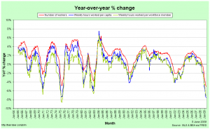
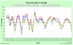
First the year-over-year % change in number of production workers, hours worked per member of the workforce and hours worked per capita:

Year-over-year changes in employment and hours worked

A casual inspection of this graph suggests that the current recession is, for employment, about the same as or a little better than the 1973-75 recession, but that is an incorrect interpretation.  This graph effectively shows rates of change, so it’s not just the depth below zero that matters but the time beneath it as well.  As we will shortly see, the current recession is actually quite a bit worse than the ’73-75 recession and the 2001 recession was a lot worse than it looks.

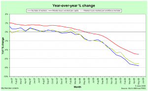
First, though, it’s instructive to zoom-in to the last year or two on the graph:

Year-over-year change in employment and hours worked (zoomed in)

The red line indicates the year-over-year change in employment.  It’s clearly badly negative.  The green line is the change in hours worked per member of the workforce.  This is worse than that for employment because not only are people losing their jobs, but those who keep their jobs are, on average, having their hours cut.  The blue line is the change in hours worked per capita.  This is the worst of the three because in addition to people losing their jobs and those with jobs having their hours cut, some of those without jobs have given up looking.  Notice that the blue and green lines were pretty close together at first.  This suggests that in the first half of the current recession, people who lost their jobs were staying in the workforce in the hope of finding work, while it was only in the second half that some of the unemployed started to lose hope and give up looking.

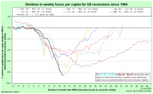
In comparing recessions, I prefer to use the hours-worked-per-capita metric because it captures much more of the employment picture than just employment figures or total hours worked.  Here is a comparison between recessions dating back to 1964, centred around their NBER-determined peak in economic activity:

Comparing hours worked per capita in US recessions relative to NBER-determined peaks in economic activity

Notice that hours worked per capita tend to have been falling for some time before the NBER-determined peak in economic activity.  This is because employment is not the be all and end all of the economy and the dating committee has to take those other elements into account as well.

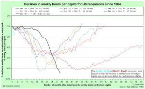
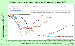
Now we rebase that comparison so each recession is relative to it’s actual peak in hours worked per capita:

Comparing US recessions relative to actual peaks in hours worked per capita

This gives us a true measure of the depth of each recession with respect to employment.  We can see that the ’71-75 and 2001 recessions reached about the same depth and that the current recession has now gone lower than either of them.  Since it is reasonable to assume that the USA will continue to lose jobs (or at least hours worked) in the next couple of months, we can safely call the current recession the worst of this group of seven.

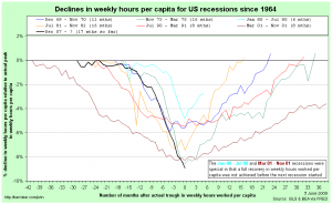
Finally, I thought it worthwhile to compare the falls relative to actual peaks, but centred around each recession’s trough in hours worked per capita (for comparison purposes, I have assumed that the current recession’s trough was in May ’09):

Comparing US recessions in hours worked per capita, centred around their troughs

This graph gives some hope to those imagining a quick recovery.  While the recoveries do tend to be a little slower than the recessions, there does appear to be some symmetry around the troughs.

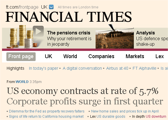
Counter-cyclical markups

One of the things that gets discussed in the currently-under-attack topic of DSGE models is that of counter-cyclical markups.  If the typical firm’s markup is counter-cyclical — that is, if it’s markup over marginal cost rises during a recession and falls during a boom — then both the magnitude and the duration of any given shock to the economy will be larger.

From the front page of the FT website this afternoon:

counter-cyclical profits

The article it’s referring to is here.

The Chrysler bankruptcy

This is not a post about how Chrysler might work going forward, nor a post about how dastardly the hold-outs are.  This is a post about the distribution of haircuts and the move from White House-led negotiation to bankruptcy court.

There are broadly four groups of creditors:  The (sole remaining) shareholder, the union/pension-fund, the bond holders and the US government.

Clearly the shareholder should be wiped out.  The question is how much of a haircut everybody else should take.

I believe that by law, the US government would take the smallest haircut (get the largest fraction of their money back) as they’re super-senior, then the bond holders in decreasing order of seniority and the union/pension fund should get the biggest kick in the teeth.  The hold-outs were secured creditors, which means that if the company is liquidated they get a pretty senior claim on the proceeds.

[Update: Duh.  The government isn’t a super-senior bond holder, it’s a preferred share holder, which means that it’s claims, in principle, ought to be subordinate to the bond holders]

As I understand it, the deal on the table had the order differently.  The unions were getting back something like 60c on the dollar, the government 45c on the dollar and the bondholders 25c on the dollar (those numbers are made-up, but indicative).

That conflict between what would normally happen and the deal on offer was what gave rise to this sort of comment from Greg Mankiw:

The Rule of Law — Not!

Via the WSJ, here is the view from a “secured (sic) creditor” of Chrysler:

“Like many others I made the mistake of buying what I believed was ‘value,'” Mr. Gwin says, adding that investors who bought at the time believed the loans were worth more than their market price. “We did not contemplate having our first liens invalidated by a sitting president,” he adds.

As the President intervenes in more and more industries, a key question is how he does it and what he is trying to achieve. Is he trying to reorganize insolvent firms while, as much as possible, preserving the rights of stakeholders as established under existing contracts? Or is he trying to achieve a “fair” outcome as he judges it, regardless of preexisting rules and agreements? I fear it may be the latter, in which case politics may start to trump the rule of law.

Mankiw has an uncanny ability to irritate me at times and although he has a bloody good point, even a vitally important point, this post did irritate me because I suspect that most bankruptcy arrangements aren’t fair, for a few reasons:

First, bond-holders, like equity holders, are ultimately speculators.  We differentiate the seniority of their claims legally, but the fact is that a guy holding a Chrysler bond is just as much of a punter as the dude holding one of the shares.  They (presumably) had the same access to information about Chrysler’s future and they (hopefully) both knew that their investment came with risk.  The idea of one subset of one factor of production being largely protected from the risk of the company’s failure is silly.

Second, employees are not speculators in the same way that the providers of capital are.  The cost of taking your money out of a company’s bonds or shares and moving it to another company is negligible.  The cost of taking your labour out and moving it to another company is significant.  At the very least, you are often geographically tied down while your money is not.  Therefore the socially optimal decision would help insure the employees against the risk of the company failing but leave the capital to insure itself.  Since US unemployment benefits (the public insurance framework) is so measly, it seems reasonable to grant employees partial access to the assets of the company.

Third, in every company to some extent (although varying depending on the industry), the employees are the company.  At an extreme, ask what a law firm would be worth if you fired all the lawyers.  Therefore, even if labour were perfectly mobile, there is a game-theoretic basis for giving the employees a stake in the game:  Principal-Agent problems exist all the way down to the floor sweepers.  This is an argument for German-style capitalism where the workers are also minority shareholders.  You might argue against workers’ representatives on the board of directors, but I do think they ought to have a share holding.

Fourth, even if all of the above balanced out to zero, there might (might!) be be beneficial social welfare to ensuring that the company is an ongoing concern rather than liquidated.  When they pushed Chrysler into bankruptcy, the hold-outs were doing so because they would get more money under liquidation than the deal on the table.  If there is a benefit to social welfare in keeping the company open, there ought to be a way to force the bond-holders to take a hefty haircut rather than liquidating the assets, even – and this is where Professor Mankiw might really get upset – if it wasn’t Pareto improving (the needs of the many …).

Nevertheless – and this is why Mankiw managed to get under my skin on this occassion – I am glad that Chrysler has gone into bankruptcy.

I am glad because even though I largely agree with the White House’s proposal, and even if my four points are all true, it is not the job of the executive to be making these decisions.    There are entire institutions set up for it.  The bankruptcy courts and the judges who preside over them specialise in this stuff.  By all means the White House might make a submission for consideration (as the executive of the country, not just as a stakeholder), but it should be up to the judge to decide.

I suspect, or at least like to imagine, that Barack Obama knows all this already (he is a constitutional lawyer, after all) and that he pushed the negotiation down the path it has taken because politically he needed to be seen to be trying to “save” Chrysler from bankruptcy and economically ne needed to avoid the market turmoil that would have ensued from a sudden move to bankruptcy rather than the tortuously gradual one we have seen.

Is America recapitalising all the non-American banks?

The recent naming of the AIG counterparties [press release, NY Times coverage] reminded me of something and this post by Brad Setser has inspired me to write on it.

Back in January, I wrote a post that contained some mistakes.  I argued that part of the reason that the M1 money multiplier in America fell below unity was because foreign banks with branches in America and American banks with branches in other countries were taking deposits from other countries and placing them in (excess) reserve at the Federal Reserve.

My first mistake was in believing that that was the only reason why the multiplier fell below one.  Of course, even if the United States were in a state of autarky it could still fall below one as all it requires is that banks withdraw from investments outside the standard definitions of money and place the proceeds in their reserve account at the Fed.

And that was certainly happening, because by paying interest on excess reserves, the Fed placed a floor under the risk-adjusted return that banks would insist on receiving for any investment.  Any position with a risk-free-equivalent yield that was less than what the Fed was paying was very rapidly unwound.

Nevertheless, I believe that my idea still applies in part.  By paying interest on excess reserves, the Fed (surely?) also placed a floor under the risk-adjusted returns for anybody with access to a US depository institution, including foreign branches of US banks and foreign banks with branches in America.  The only difference is that those groups would also have had exchange-rate risk to incorporate.  But since the US dollar enjoys reserve currency status, it may have seemed a safe bet to assume that the USD would not fall while the money was in America at the Fed because of the global flight to quality.

The obvious question is to then ask how much money held in (excess) reserve at the Fed originated from outside of America.  Over 2008:Q4, the relevant movements were: [1]

Remember that, roughly speaking, the definitions are:

  • monetary base = currency + required reserves + excess reserves
  • m1 = currency + demand deposits

So we can infer that next to the $707 billion increase in excess reserves, demand deposits only increased by $148 billion and required reserves by $7 billion.

In a second mistake in my January post, I thought that it was the difference in growth between m1 and the monetary base that needed explaining.  That was silly.  Strictly speaking it is the entirety of the excess reserve growth that we want to explain.  How much was from US banks unwinding domestic positions and how much was from foreigners?

Which is where we get to Brad’s post.  In looking at the latest Flow of Funds data from the Federal Reserve, he noted with some puzzlement that over 2008:Q4 for the entire US banking system (see page 69 of the full pdf):

  • liabilities to domestic banks (floats and discrepancies in interbank transactions) went from $-50.9 billion to $-293.4 billion.
  • liabilities to foreign banks went from $-48.1 billion to $289.5 billion

I’m not sure about the first of those, but on the second that represents a net loan of $337.6 billion from foreign banks to US banks over that last quarter.

Could that be foreign banks indirectly making use of the Fed’s interest payments on excess reserves?

No matter what the extent of foreign banks putting money in reserve with the Fed, that process – together with the US government-backed settlements of AIGs foolish CDS contracts – amounts to America (partially) recapitalising not just its own, but the banking systems of the rest of the world too.

[1] M1 averaged 1435.1 in September and 1624.7 in December.  Monetary base averaged 936.138 in September and 1692.511 in December.  Currency averaged 776.7 in September and 819.0 in December. Excess reserves averaged 60.051 in September and 767.412 in December.  Remember that the monthly figures released by the Federal Reserve are dated at the 1st of the month but are actually an average for the whole of the month.

US February Employment and Recession vs. Depression

The preliminary employment data for February in the USA has been out for a little while now and I thought it worthwhile to update the graphs I did after January’s figures.

As I explained when producing the January graphs, I believe that it’s more representative to look at Weekly Hours Worked Per Capita than at just the number of people with jobs so as to more fully take into account part-time work, the entry of women into the labour force and the effects of discouraged workers.  Graphs that only look at total employment (for example: 1, 2) paint a distorted picture.

The Year-over-Year percentage changes in the number of employed workers, the weekly hours per capita and the weekly hours per workforce member continue to worsen.  The current recession is still not quite as bad as that in 1981/82 by this measure, but it’s so close as to make no difference.

Year-over-year changes in employment and hours worked

Just looking at year-over-year figures is a little deceptive, though, as it’s not just how far below the 0%-change line you fall that matters, but also how long you spend below it.  Notice, for example, that while the 2001 recession never saw catastrophically rapid falls in employment, it continued to decline for a remarkably long time.

That’s why it’s useful to compare recessions in terms of their cumulative declines from peak:

Comparing US recessions relative to actual peaks in weekly hours worked per capitaA few points to note:

  • The figures are relative to the actual peak in weekly hours worked per capita, not to the official (NBER-determined) peak in economic activity.
  • I have shown the official recession durations (solid arrows) and the actual periods of declining weekly hours worked per capita (dotted lines) at the top.
  • The 1980 and 2001 recessions were odd in that weekly hours worked per capita never fully recovered before the next recession started.

The fact that the current recession isn’t yet quite as bad as the 1981/82 recession is a little clearer here.  The 1973-75 recession stands out as being worse than the current one and the 2001 recession was clearly the worst of all.

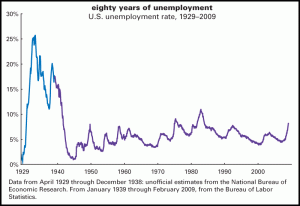
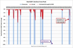
There’s also some question over the US is actually in a depression rather than just a recession.  The short answer is no, or at least not yet.  There is no official definition of a depression, but a cumulative decline of 10% in real GDP is often bandied around as a good rule of thumb.  Here are two diagrams that illustrate just how much worse things would need to be before the US was really in a depression …

First, from The Liscio Report, we have an estimated unemployment rate time-series that includes the Great Depression:

Historic Unemployment Rates in the USA

Second, from Calculated Risk, we have a time-series of cumulative declines in real gdp since World War II:

Cumulative declines in real GDP (USA)

Remember that we’d need to fall to -10% to hit the common definition of a depression.

Evil

Evil, I say:

Dozens of specially trained agents work on the third floor of DCM Services here, calling up the dear departed’s next of kin and kindly asking if they want to settle the balance on a credit card or bank loan, or perhaps make that final utility bill or cellphone payment.

The people on the other end of the line often have no legal obligation to assume the debt of a spouse, sibling or parent. But they take responsibility for it anyway.

Evil.

How to value toxic assets (part 6)

Via Tyler Cowen, I am reminded (again) that I should really be reading Steve Waldman more often.  Like, all the time.  After reading John Hempton’s piece that I highlighted last time, Waldman writes, as an afterthought:

There’s another way to generate price transparency and liquidity for all the alphabet soup assets buried on bank balance sheets that would require no government lending or taxpayer risk-taking at all. Take all the ABS and CDOs and whatchamahaveyous, divvy all tranches into $100 par value claims, put all extant information about the securities on a website, give ’em a ticker symbol, and put ’em on an exchange. I know it’s out of fashion in a world ruined by hedge funds and 401-Ks and the unbearable orthodoxy of index investing. But I have a great deal of respect for that much maligned and nearly extinct species, the individual investor actively managing her own account. Individual investors screw up, but they are never too big to fail. When things go wrong, they take their lumps and move along. And despite everything the professionals tell you, a lot of smart and interested amateurs could build portfolios that match or beat the managers upon whose conflicted hands they have been persuaded to rely. Nothing generates a market price like a sea of independent minds making thousands of small trades, back and forth and back and forth.

I don’t really expect anybody to believe me, but I’ve been thinking something similar.

CDOs, CDOs-squared and all the rest are derrivatives that are traded over the counter; that is, they are traded entirely privately.  If bank B sells some to hedge fund Y, nobody else finds out any details of the trade or even that the trade took place.  The closest we come is that when bank B announces their quarterly accounts, we might realise that they off-loaded some assets.

On the more popularly known stock and bond markets, buyers publicly post their “bid” prices and sellers post their “ask” prices. When the prices meet, a trade occurs.[*1] Most details of the trade are then made public – the price(s), the volume, the particular details of the asset (ordinary shares in XXX, 2-year senior notes from XXX with an expiry of xx/xx/xxxx, etc) – everything except the identity of the buyer and seller. Those details then provide some information to everybody watching on how the buyer and seller value the asset. Other market players can then combine that with their own private valuations and update their own bid or ask prices accordingly. In short, the market aggregates information. [*2]

When assets are traded over the counter (OTC), each participant can only operate on their private valuation. There is no way for the market to aggregate information in that situation. Individual banks might still partially aggregate information by making a lot of trades with a lot of other institutions, since each time they trade they discover a bound on the valuation of the other party (an upper bound when you’re buying and the other party is selling, a lower bound when you’re selling and they’re buying).

To me, this is a huge failure of regulation. A market where information is not publicly and freely available is an inefficient market, and worse, one that expressly creates an incentive for market participants to confuse, conflate, bamboozle and then exploit the ignorant. Information is a true public good.

On that basis, here is my idea:

Introduce new regulation that every financial institution that wants to get support from the government must anonymously publish all details of every trade that they’re party to. The asset type, the quantity, the price, any time options on the deal, everything except the identity of the parties involved. Furthermore, the regulation would be retroactive for X months (say, two years, so that we get data that predates the crisis).  On top of that, the regulation would require that every future trade from everyone (whether they were receiving government assistance or not) would be subject to the same requirementes.  Then everything acts pretty much like the stock and bond markets.

The latest edition of The Economist has an article effectively questioning whether this is such a good idea.

[T]ransparency and liquidity are close relatives. One enemy of liquidity is “asymmetric information”. To illustrate this, look at a variation of the “Market for Lemons” identified by George Akerlof, a Nobel-prize-winning economist, in 1970. Suppose that a wine connoisseur and Joe Sixpack are haggling over the price of the 1998 Château Pétrus, which Joe recently inherited from his rich uncle. If Joe and the connoisseur only know that it is a red wine, they may strike a deal. They are equally uninformed. If vintage, region and grape are disclosed, Joe, fearing he will be taken for a ride, may refuse to sell. In financial markets, similarly, there are sophisticated and unsophisticated investors, and unless they have symmetrical information, liquidity can dry up. Unfortunately transparency may reduce liquidity. Symmetry, not the amount of information, matters.

I’m completely okay with this. Symmetric access to information and symmetric understanding of that information is the ideal. From the first paragraph and then the last paragraph :

… Not long ago the cheerleaders of opacity were the loudest. Without privacy, they argued, financial entrepreneurs would be unable to capture the full value of their trading strategies and other ingenious intellectual property. Forcing them to disclose information would impair their incentive to uncover and correct market inefficiencies, to the detriment of all …

Still, for all its difficulties, transparency is usually better than the alternative. The opaque innovations of the recent past, rather than eliminating market inefficiencies, unintentionally created systemic risks. The important point is that financial markets are not created equal: they may require different levels of disclosure. Liquidity in the stockmarket, for example, thrives on differences of opinion about the value of a firm; information fuels the debate. The money markets rely more on trust than transparency because transactions are so quick that there is little time to assess information. The problem with hedge funds is that a lack of information hinders outsiders’ ability to measure their contribution to systemic risk. A possible solution would be to impose delayed disclosure, which would allow the funds to profit from their strategies, provide data for experts to sift through, and allay fears about the legality of their activities. Transparency, like sunlight, needs to be looked at carefully.

This strikes me as being around the wrong way.  Money markets don’t rely on trust because their transactions are so fast; their transactions are so fast because they’re built on trust.  The scale of the crisis can be blamed, in no small measure, because of the breakdown in that trust.

I also do not buy the idea of opacity begetting market efficiency.  It makes no sense.  The only way that information disclosure can remove the incentive to “uncover and correct” inefficiencies in the market is if by making the information public you reduce the inefficiency.  I’m not suggesting that we force market participants to reveal what they discover before they get the chance to act on it.  I’m only suggesting that the details of their action should be public.

[*1] Okay, it’s not exactly like that, but it’s close enough.

[*2] Note that information aggregation does not necessarily imply that the Efficient Market Hypothesis (EMH), but the EMH requires information aggregation to work.

Other posts in this series:  1, 2, 3, 4, 5, [6].

From tacit to (almost) explicit: inflation targetting at the Fed

From the latest press release of the US Federal Reserve Board:

The central tendency of FOMC participants’ longer-run projections, submitted for the Committee’s January 27-28 meeting, were:

  • 2.5 to 2.7 percent growth in real gross domestic output
  • 4.8 to 5.0 percent unemployment
  • 1.7 to 2.0 percent inflation, as measured by the price index for personal consumption expenditures (PCE).

Most participants judged that a longer-run PCE inflation rate of 2 percent would be consistent with the dual mandate; others indicated that 1-1/2 or 1-3/4 percent inflation would be appropriate.

Speaking earlier in the day, Fed Chairman Ben Bernanke observed:

These longer-term projections will inform the public of the Committee participants’ estimates of the rate of growth of output and the unemployment rate that appear to be sustainable in the long run in the United States, taking into account important influences such as the trend growth rates of productivity and the labor force, improvements in worker education and skills, the efficiency of the labor market at matching workers and jobs, government policies affecting technological development or the labor market, and other factors. The longer-term projections of inflation may be interpreted, in turn, as the rate of inflation that FOMC participants see as most consistent with the dual mandate given to it by the Congress–that is, the rate of inflation that promotes maximum sustainable employment while also delivering reasonable price stability.

(Hat tip: Calculated Risk)

How to value toxic assets (part 5)

John Hempton has an excellent post on valuing the assets on banks’ balance sheets and whether banks are solvent.  He starts with a simple summary of where we are:

We have a lot of pools of bank assets (pools of loans) which have the following properties:
  • The assets sit on the bank’s balance sheet with a value of 90 – meaning they have either being marked down to 90 (say mark to mythical market or model) or they have 10 in provisions for losses against them.
  • The same assets when they run off might actually make 75 – meaning if you run them to maturity or default the bank will – discounted at a low rate – recover 75 cents in the dollar on value.

The banks are thus under-reserved on an “held to maturity” basis. Heavily under-reserved.

He then gives another explanation (on top of the putting-Humpty-Dumpty-back-together-again idea I mentioned previously) of why the market price is so far below the value that comes out of standard asset pricing:

Before you go any further you might wonder why it is possible that loans that will recover 75 trade at 50? Well its sort of obvious – in that I said that they recover 75 if the recoveries are discounted at a low rate. If I am going to buy such a loan I probably want 15% per annum return on equity.

The loan initially yielded say 5%. If I buy it at 50 I get a running yield of 10% – but say 15% of the loans are not actually paying that yield – so my running yield is 8.5%. I will get 75-80c on them in the end – and so there is another 25cents to be made – but that will be booked with an average duration of 5 years – so another 5% per year. At 50 cents in the dollar the yield to maturity on those bad assets is about 15% even though the assets are “bought cheap”. That is not enough for a hedge fund to be really interested – though if they could borrow to buy those assets they might be fun. The only problem is that the funding to buy the assets is either unavailable or if available with nasty covenants and a high price. Essentially the 75/50 difference is an artefact of the crisis and the unavailability of funding.

The difference between the yield to maturity value of a loan and its market value is extremely wide. The difference arises because you can’t eaily borrow to fund the loans – and my yield to maturity value is measured using traditional (low) costs of funds and market values loans based on their actual cost of funds (very high because of the crisis).

The rest of Hempton’s piece speaks about various definitions of solvency, whether (US) banks meet each of those definitions and points out the vagaries of the plan recently put forward by Geithner.  It’s all well worth reading.

One of the other important bits:

Few banks would meet capital adequacy standards. Given the penalty for even appearing as if there was a chance that you would not meet capital adequacy standards is death (see WaMu and Wachovia) and this is a self-assessed exam, banks can be expected not to tell the truth.

(It was Warren Buffett who first – at least to my hearing – described financial accounts as a self-assessed exam for which the penalty for failure is death. I think he was talking about insurance companies – but the idea is the same. Truth is not expected.)

Other posts in this series:  1, 2, 3, 4, [5], 6.

Perspective (Comparing Recessions)

This is quite a long post.  I hope you’ll be patient and read it all – there are plenty of pretty graphs!

I have previously spoken about the need for some perspective when looking at the current recession.  At the time (early Dec 2008), I was upset that every regular media outlet was describing the US net job losses of 533k in November as being unprecedentedly bad when it clearly wasn’t.

About a week ago, the office of Nancy Pelosi (the Speaker of the House of Representatives in the US) released this graph, which makes the current recession look really bad:
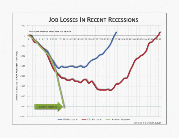
Notice that a) the vertical axis lists the number of jobs lost and b) it only includes the last three recessions.  Shortly afterward, Barry Ritholtz posted a graph that still had the total number of jobs lost on the vertical axis, but now included all post-World War Two recessions:
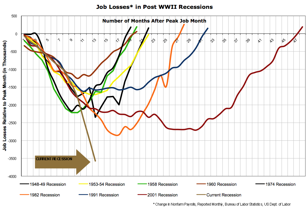
Including all the recessions is an improvement if only for the sake of context, but displaying total job losses paints a false picture for several reasons:

  1. Most importantly, it doesn’t allow for increases in the population.  The US residential population in 1974 was 213 million, while today it is around 306 million.  A loss of 500 thousand jobs in 1974 was therefore a much worse event than it is today.
  2. Until the 1980s, most households only had one source of labour income.  Although the process started slowly much earlier, in the 1980s very large numbers of women began to enter the workforce, meaning that households became more likely to have two sources of labour income.  As a result, one person in a household losing their job is not as catastrophic today as it used to be.
  3. There has also been a general shift away from full-time work and towards part-time work.  Only looking at the number of people employed (or, in this case, fired) means that we miss altogether the impact of people having their hours reduced.
  4. We should also attempt to take into account discouraged workers; i.e. those who were unemployed and give up even looking for a job.

Several people then allowed for the first of those problems by giving graphs of job loses as percentages of the employment level at the peak of economic activity before the recession.  Graphs were produced, at the least, by Justin Fox, William Polley and Calculated Risk.  All of those look quite similar.  Here is Polley’s:
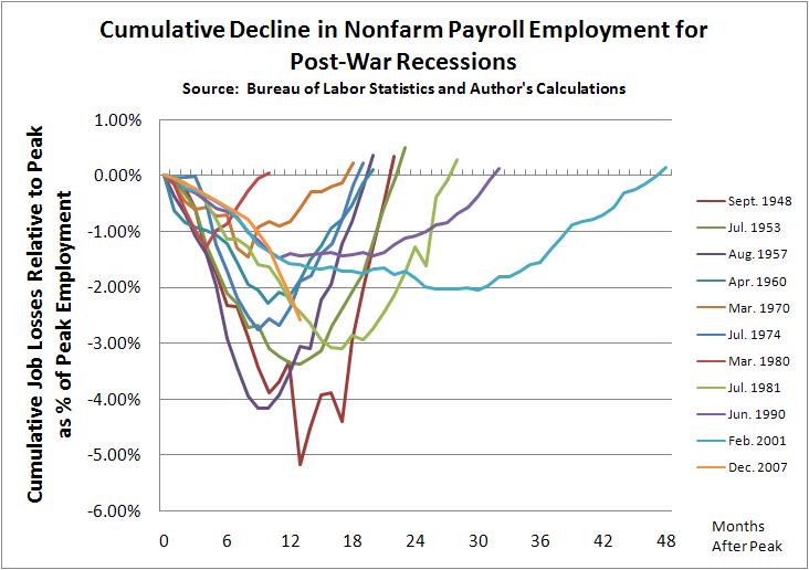
The current recession is shown in orange.  Notice the dramatic difference to the previous two graphs?  The current recession is now shown as being quite typical; painful and worse than the last two recessions, but entirely normal.  However, this graph is still not quite right because it still fails to take into account the other three problems I listed above.

(This is where my own efforts come in)

The obvious way to deal with the rise of part-time work is to graph (changes in) hours worked rather than employment.

The best way to also deal with the entry of women into the workforce is to graph hours worked per member of the workforce or per capita.

The only real way to also (if imperfectly) account for discouraged workers is to just graph hours worked per capita (i.e. to compare it to the population as a whole).

This first graph shows Weekly Hours Worked per capita and per workforce member since January 1964:
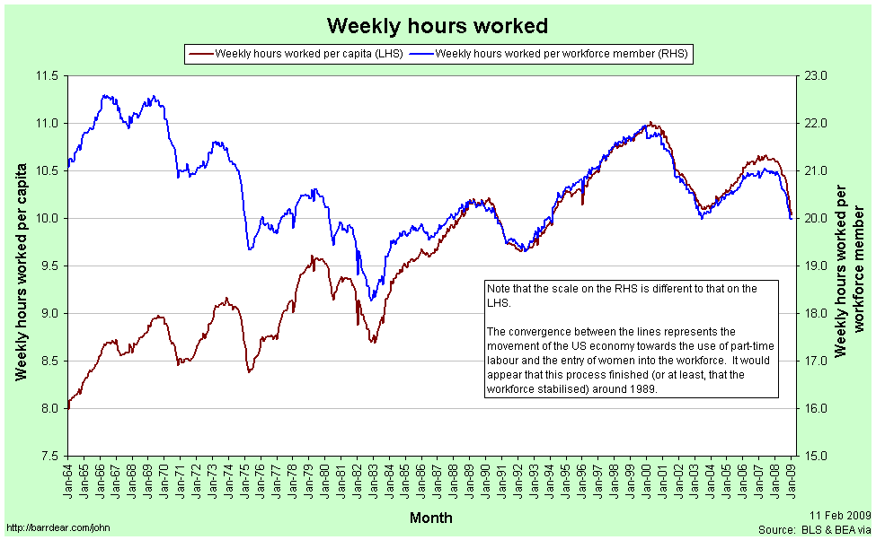
In January 1964, the average member of the workforce worked just over 21 hours per week.  In January 2009 they worked just under 20 hours per week.

The convergence between the two lines represents the entry of women into the workforce (the red line is increasing) and the increasing prevalence of part-time work (the blue line is decreasing).  Each of these represented a structural change in the composition of the labour force.  The two processes appear to have petered out by 1989. Since 1989 the two graphs have moved in tandem.

[As a side note: In econometrics it is quite common to look for a structural break in some timeseries data.  I’m sure it exists, but I am yet to come across a way to rigorously handle the situation when the “break” takes decades occur.]

The next graph shows Year-over-Year percentage changes in the number of employed workers, the weekly hours per capita and the weekly hours per workforce member:
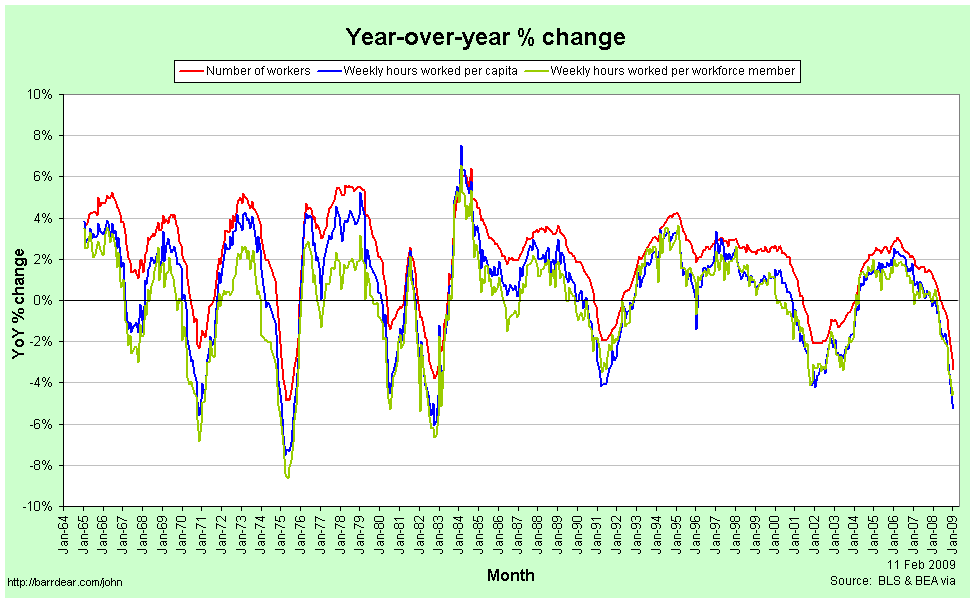
Note that changes in the number of workers are consistently higher than the number of hours per workforce member or per capita.  In a recession, people are not just laid off, but the hours that the remaining employees are given also falls, so the average number of hours worked falls much faster.  In a boom, total employment rises faster than the average number of hours, meaning that the new workers are working few hours than the existing employees.

This implies that the employment situation faced by the average individual is consistently worse than we might think if we restrict our attention to just the number of people in any kind of employment.  In particular, it means that from the point of view of the average worker, recessions start earlier, are deeper and last longer than they do for the economy as a whole.

Here is the comparison of recessions since 1964 from the point of view of Weekly Hours Worked per capita, with figures relative to those in the month the NBER determines to be the peak of economic activity:
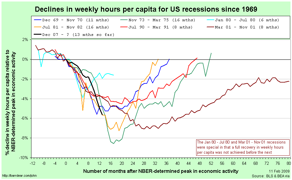
The labels for each line are the official (NBER-determined) start and end dates for the recession.  There are several points to note in comparing this graph to those above:

  • The magnitudes of the declines are considerably worse than when simply looking at aggregate employment.
  • Declines in weekly hours worked per capita frequently start well before the NBER-determined peak in economic activity.  For the 2001 recession, the decline started 11 months before the official peak.
  • For two recessions out of the last seven – those in 1980 and 2001 – the recovery never fully happened; another recession was deemed to have started before the weekly hours worked climbed back to its previous peak.
  • The 2001 recession was really awful.
  • The current recession would appear to still be typical.

Since so many of the recessions started – from the point of view of the average worker – before the NBER-determined date, it is helpful to rebase that graph against the actual peak in weekly hours per capita:
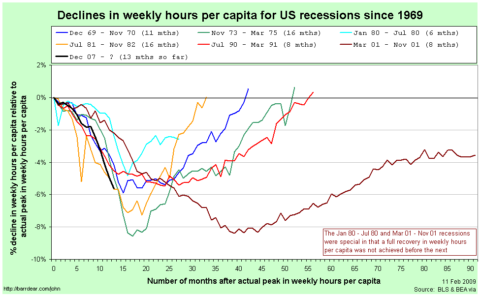
Now, finally, we have what I believe is an accurate comparison of the employment situation in previous recessions.

Once again, the labels for each line are the official (NBER-determined) start and end dates for the recession.  By this graph, the 2001 recession is a clear stand-out.  It fell the second furthest (and almost the furthest), lasted by far the longest and the recovery never fully happened.

The current recession also stands out as being toward the bad end of the spectrum.  It is the equally worst recession by this point since the peak.  It will need to continue getting a lot worse quite quickly in order to maintain that record, however.

After seeing Calculated Risk’s graph, Barry Ritholtz asked whether it is taking longer over time to recover from a recession recoveries (at least in employment).  This graph quite clearly suggests that the answer is “no.”  While the 2001 and 1990/91 recessions do have the slowest recoveries, the next two longest are the earliest.

Perhaps a better way to characterise it is to compare the slope coming down against the slope coming back up again.  It seems as a rough guess that rapid contractions are followed by just-as-rapid rises.  On that basis, at least, we have some slight cause for optimism.

If anybody is interested, I have also uploaded a copy of the spreadsheet with all the raw data for these graphs.  You can access it here:  US Employment (excel spreadsheet)

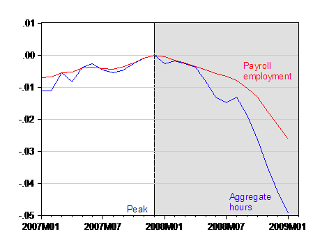
For reference, the closest other things that I have seen to this presentation in the blogosphere are this post by Spencer at Angry Bear and this entry by Menzie Chinn at EconBrowser.  He provides this graph of employment versus aggregate hours for the current recession only:
Alex Tabarrok has also been comparing recessions (1, 2, 3).