In which I respectfully disagree with Paul Krugman

Paul Krugman [Ideas, Princeton, Unofficial archive] has recently started using the phrase “jobless recovery” to describe what appears to be the start of the economic recovery in the United States [10 Feb, 21 Aug, 22 Aug, 24 Aug].  The phrase is not new.  It was first used to describe the recovery following the 1990/1991 recession and then used extensively in describing the recovery from the 2001 recession.  In it’s simplest form, it is a description of an economic recovery that is not accompanied by strong jobs growth.  Following the 2001 recession, in particular, people kept losing jobs long after the economy as a whole had reached bottom and even when employment did bottom out, it was very slow to come back up again.  Professor Krugman (correctly) points out that this is a feature of both post-1990 recessions, while prior to that recessions and their subsequent recoveries were much more “V-shaped”.  He worries that it will also describe the recovery from the current recession.

While Professor Krugman’s characterisations of recent recessions are broadly correct, I am still inclined to disagree with him in predicting what will occur in the current recovery.  This is despite Brad DeLong’s excellent advice:

  1. Remember that Paul Krugman is right.
  2. If your analysis leads you to conclude that Paul Krugman is wrong, refer to rule #1.

This will be quite a long post, so settle in.  It’s quite graph-heavy, though, so it shouldn’t be too hard to read. 🙂

Professor Krugman used his 24 August post on his blog to illustrate his point.  I’m going to quote most of it in full, if for no other reason than because his diagrams are awesome:

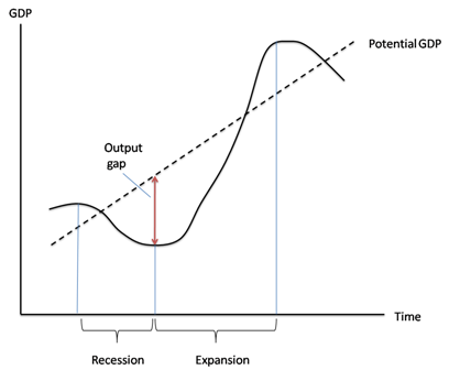
First, here’s the standard business cycle picture:

DESCRIPTION

Real GDP wobbles up and down, but has an overall upward trend. “Potential output” is what the economy would produce at “full employment”, which is the maximum level consistent with stable inflation. Potential output trends steadily up. The “output gap” — the difference between actual GDP and potential — is what mainly determines the unemployment rate.

Basically, a recession is a period of falling GDP, an expansion a period of rising GDP (yes, there’s some flex in the rules, but that’s more or less what it amounts to.) But what does that say about jobs?

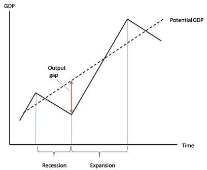
Traditionally, recessions were V-shaped, like this:

DESCRIPTION

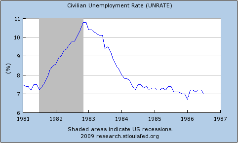
So the end of the recession was also the point at which the output gap started falling rapidly, and therefore the point at which the unemployment rate began declining. Here’s the 1981-2 recession and aftermath:

DESCRIPTION

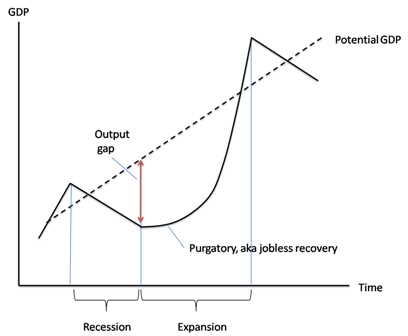
Since 1990, however, growth coming out of a slump has tended to be slow at first, insufficient to prevent a widening output gap and rising unemployment. Here’s a schematic picture:

DESCRIPTION

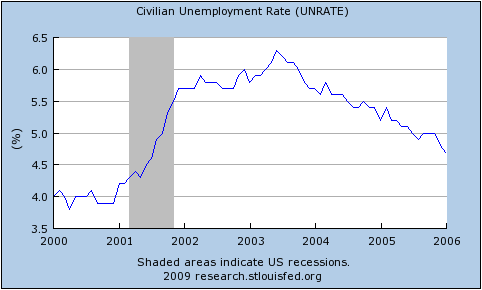
And here’s the aftermath of the 2001 recession:

DESCRIPTION

Notice that this is NOT just saying that unemployment is a lagging indicator. In 2001-2003 the job market continued to get worse for a year and a half after GDP turned up. The bad times could easily last longer this time.

Before I begin, I have a minor quibble about Prof. Krugman’s definition of “potential output.”  I think of potential output as what would occur with full employment and no structural frictions, while I would call full employment with structural frictions the “natural level of output.”  To me, potential output is a theoretical concept that will never be realised while natural output is the central bank’s target for actual GDP.  See this excellent post by Menzie Chinn.  This doesn’t really matter for my purposes, though.

In everything that follows, I use total hours worked per capita as my variable since that most closely represents the employment situation witnessed by the average household.  I only have data for the last seven US recessions (going back to 1964).  You can get the spreadsheet with all of my data here: US_Employment [Excel].  For all images below, you can click on them to get a bigger version.

The first real point I want to make is that it is entirely normal for employment to start falling before the official start and to continue falling after the official end of recessions.  Although Prof. Krugman is correct to point out that it continued for longer following the 1990/91 and 2001 recessions, in five of the last six recessions (not counting the current one) employment continued to fall after the NBER-determined trough.  As you can see in the following, it is also the case that six times out of seven, employment started falling before the NBER-determined peak, too.

Hours per capita fell before and after recessions

Prof. Krugman is also correct to point out that the recovery in employment following the 1990/91 and 2001 recessions was quite slow, but it is important to appreciate that this followed a remarkably slow decline during the downturn.  The following graph centres each recession around it’s actual trough in hours worked per capita and shows changes relative to those troughs:

Hours per capita relative to and centred around trough

The recoveries following the 1990/91 and 2001 recessions were indeed the slowest of the last six, but they were also the slowest coming down in the first place.  Notice that in comparison, the current downturn has been particularly rapid.

We can go further:  the speed with which hours per capita fell during the downturn is an excellent predictor of how rapidly they rise during the recovery.  Here is a scatter plot that takes points in time chosen symmetrically about each trough (e.g. 3 months before and 3 months after) to compare how far hours per capita fell over that time coming down and how far it had climbed on the way back up:

ComparingRecessions_20090605_Symmetry_Scatter_All

Notice that for five of the last six recoveries, there is quite a tight line describing the speed of recovery as a direct linear function of the speed of the initial decline.  The recovery following the 1981/82 recession was unusually rapid relative to the speed of it’s initial decline.  Remember (go back up and look) that Prof. Krugman used the 1981/82 recession and subsequent recovery to illustrate the classic “V-shaped” recession.  It turns out to have been an unfortunate choice since that recovery was abnormally rapid even for pre-1990 downturns.

Excluding the 1981/82 recession on the basis that it’s recovery seems to have been driven by a separate process, we get quite a good fit for a simple linear regression:

ComparingRecessions_20090605_Symmetry_Scatter_Excl_81-82

Now, I’m the first to admit that this is a very rough-and-ready analysis.  In particular, I’ve not allowed for any autoregressive component to employment growth during the recovery.  Nevertheless, it is quite strongly suggestive.

Given the speed of the decline that we have seen in the current recession, this points us towards quite a rapid recovery in hours worked per capita (although note that the above suggests that all recoveries are slower than the preceding declines – if they were equal, the fitted line would be at 45% (the coefficient would be one)).

Article Summary: Noisy Directional Learning and the Logit Equilibrium

The paper is here (ungated).  The ideas.repec entry is here.  I believe that this (1999) was an early version of the same.  The authors are Simon P. Anderson [Ideas, Virginia] , Jacob K. Goeree [Ideas, CalTech] and Charles A. Holt [Ideas, Virginia].  The full reference is:

Anderson, Simon P.; Goeree, Jacob K. and Holt, Charles A., “Noisy Directional Learning and the Logit Equilibrium.” Scandinavian Journal of Economics, Special Issue in Honor of Reinhard Selten, 2004, 106(3), pp. 581-602, September 2004

The abstract:

We specify a dynamic model in which agents adjust their decisions toward higher payoffs, subject to normal error. This process generates a probability distribution of players’ decisions that evolves over time according to the Fokker–Planck equation. The dynamic process is stable for all potential games, a class of payoff structures that includes several widely studied games. In equilibrium, the distributions that determine expected payoffs correspond to the distributions that arise from the logit function applied to those expected payoffs. This ‘‘logit equilibrium’’ forms a stochastic generalization of the Nash equilibrium and provides a possible explanation of anomalous laboratory data.

This is a model of bounded rationality inspired, in part, by experimental results.  It provides a stochastic equilibrium (i.e. a distribution over choices) that need not coincide with, nor even be centred around, the Nash equilibrium.  The summary is below the fold.

Continue reading “Article Summary: Noisy Directional Learning and the Logit Equilibrium”

A question for behavioural economists

How true is the old adage “easy come, easy go”?  More formally, is it fair to suggest that an individual’s marginal propensity to consume (MPC) — the share of an extra dollar of income that they would spend on consumption rather than save — depends on the origin of the income?  The traditional wisdom would suggest that:

MPC (fortuitous income) > MPC (hard-earned income)

Have there been any studies on this?  If so, have there been any studies that apply the results to the evolution of US inequality in income and consumption?

The short-long-run, the medium-long-run and the long-long-run

EC102 has once again finished for the year.  It occurs to me that my students (quite understandably) got a little confused about the timeframes over which various elements of macroeconomics occur.  I think the reason is that we use overlapping ideas of medium- and long-run timeframes.

In essense, there are four models that we use at an undergraduate level for thinking about aggregate demand and supply.  In increasing order of time-spans involved, they are:  Investment & Savings vs. Liquidity & Money (IS-LM),  Aggregate Supply – Aggregate Demand (AS-AD), Factor accumulation (Solow growth), and Endogenous Growth Theory.

It’s usually taught that following an exogenous shock, the IS-LM model reaches a new equilibrium very quickly (which means that the AD curve shifts very quickly), the goods market in the AS-AD world clears quite quickly and the economy returns to full-employment in “the long-run” once all firms have a chance to update their prices.

But when thinking about the Solow growth model of factor (i.e. capital) accumulation, we often refer to deviations from the steady-state being in the medium-run and that we reach the steady state in the long-run.  This is not the same “long-run” as in the AS-AD model.  The Solow growth model is a classical model, which among other things means that it assumes full employment all the time.  In other words, the medium-run in the world of Solow is longer than the long-run of AS-AD.  The Solow growth model is about shifting the steady-state of the AS-AD model.

Endogenous growth theory then does the same thing to the Solow growth model: endogenous growth is the shifting of the steady-state in a Solow framework.

What we end up with are three different ideas of the “long-run”:  one at business-cycle frequencies, one for catching up to industrialised nations and one for low-frequency stuff in the industrialised countries, or as I like to call them: the short-long-run, the medium-long-run and the long-long-run.

Counter-cyclical markups

One of the things that gets discussed in the currently-under-attack topic of DSGE models is that of counter-cyclical markups.  If the typical firm’s markup is counter-cyclical — that is, if it’s markup over marginal cost rises during a recession and falls during a boom — then both the magnitude and the duration of any given shock to the economy will be larger.

From the front page of the FT website this afternoon:

counter-cyclical profits

The article it’s referring to is here.

Negative productivity shocks are conceptually okay when applied idiosyncratically to labour

This is mostly a note to myself.

Way back in the dawn of the modern-macro era, the fresh-water Chicago kids came up with Real Business Cycle theory where they endogenised the labour supply and claimed that macro variation was explained by productivity shocks.

The salt-water gang then accepted the techniques of RBC but proposed a bunch of demand-side shocks instead.

The big criticism of productivity shocks has always been to ask how you can realistically get negative shocks to productivity.  Technological regress just doesn’t seem all that likely.

Now, models of credit cycles like Kiotaki (1998) show how a small and temporary negative shock to productivity can turn into a large and persistent downturn in the economy.  In short:  Credit constraints mean that some wealth remains in the hands of the unproductive instead of being lent to the productive sectors of the economy.  The share of wealth owned by the productive is therefore a factor in aggregate output.  A temporary negative shock to productivity keeps more of the wealth with the unproductive for production purposes and it takes time for the productive sector to accumulate its wealth back.  If some sort of physical capital (e.g. land) is used as collateral, the shock will also lower the price of the capital, thus decreasing the value of the collateral and so imposing tighter restrictions on credit.

But Kiyotaki’s model still requires some productive regress …

Looking at Aiyagari (1994) and Castaneda, Diaz-Gimenez and Rios-Rull (2003) today (lecture 3 by Michaelides in EC442), I realise that small negative productivity shocks are conceptually okay if they’re applied idiosyncratically (i.e. individually) to labour.

Let s_{t} be your efficiency state in period ts is a Markov process with transition matrix \Gamma_{ss}e\left(s\right) is the efficiency of somebody in state s.  Castaneda, Diaz-Gimenez and Rios-Rull use this calibration, taken from the data:

State s=1 s=2 s=3 s=4
e(s) 1.00 3.15 9.78 1,061.00
Share of population 61.1% 22.35% 16.50% 0.05%

The transition matrix would be such that the population-shares for each state are stationary.

A household’s labour income is then given by e(s)wl.

A movement from s=3 to s=2, say, is therefore a negative labour productivity shock for the household.

The trick is to think of the efficiency states as job positions. Somebody moving from s=3 to s=1 is losing their job as an engineer and getting a job as an office cleaner.  They will probably increase l to partially compensate for the lose in hourly wage (e\left(s\right)w).

Remember that in the (Neo/New) Classical models, there’s an assumption of zero unemployment.  However much you want to work, that’s how much you work.  [That might sound silly to a casual reader, but it’s okay as a first approximation.  There are (i.e. search-and-matching) models out there that look at unemployment and can be fitted into this framework.]

If everybody is equally good at every job position (as we have here) and all the idiosyncratic shocks balance out so the population shares are constant, then – I believe – there shouldn’t be any change in observed aggregate productivity.

However, if you introduced imperfect transfer of ability across positions so that efficiency becomes e\left(s,\theta\left(s\right)\right) where \theta\left(s\right) is your private type per job position, then idiosyncratic shocks could therefore show up in aggregate numbers.

This is essentially an idea of mismatching.  A senior engineering job is destroyed and a draftsman job is created both in Detroit, while the opposite occurs in Washington state.  Since the engineer in Detroit can’t easily move to Washington, he takes the lower-productivity job and a sub-optimal person gets promoted in Washington.

Article Summary: Economics and Identity

You can access the published paper here and the unpublished technical appendices here.  The authors are George Akerlof [Ideas, Berkeley] and Rachel Kranton [Duke University].  The full reference is:

Akerlof, George A. and Kranton, Rachel E. “Economics and Identity.” Quarterly Journal of Economics, 2000, 115(3), pp. 715-53.

The abstract:

This paper considers how identity, a person’s sense of self, affects economic outcomes.We incorporate the psychology and sociology of identity into an economic model of behavior. In the utility function we propose, identity is associated with different social categories and how people in these categories should behave. We then construct a simple game-theoretic model showing how identity can affect individual interactions.The paper adapts these models to gender discrimination in the workplace, the economics of poverty and social exclusion, and the household division of labor. In each case, the inclusion of identity substantively changes conclusions of previous economic analysis.

I’m surprised that this paper was published in such a highly ranked economics journal.  Not because of a lack of quality in the paper, but because of it’s topic.  It reads like a sociology or psychology paper.  99% of the mathematics were banished to the unpublished appendices, while what made it in were the justifications by “real world” examples.  The summary is below the fold … Continue reading “Article Summary: Economics and Identity”

Is economics looking at itself?

Patricia Cowen recently wrote a piece for the New York Times:  “Ivory Tower Unswayed by Crashing Economy

The article contains precisely what you might expect from a title like that.  This snippet gives you the idea:

The financial crash happened very quickly while “things in academia change very, very slowly,” said David Card, a leading labor economist at the University of California, Berkeley. During the 1960s, he recalled, nearly all economists believed in what was known as the Phillips curve, which posited that unemployment and inflation were like the two ends of a seesaw: as one went up, the other went down. Then in the 1970s stagflation — high unemployment and high inflation — hit. But it took 10 years before academia let go of the Phillips curve.

James K. Galbraith, an economist at the Lyndon B. Johnson School of Public Affairs at the University of Texas, who has frequently been at odds with free marketers, said, “I don’t detect any change at all.” Academic economists are “like an ostrich with its head in the sand.”

“It’s business as usual,” he said. “I’m not conscious that there is a fundamental re-examination going on in journals.”

Unquestioning loyalty to a particular idea is what Robert J. Shiller, an economist at Yale, says is the reason the profession failed to foresee the financial collapse. He blames “groupthink,” the tendency to agree with the consensus. People don’t deviate from the conventional wisdom for fear they won’t be taken seriously, Mr. Shiller maintains. Wander too far and you find yourself on the fringe. The pattern is self-replicating. Graduate students who stray too far from the dominant theory and methods seriously reduce their chances of getting an academic job.

My reaction is to say “Yes.  And No.”  Here, for example, is a small list of prominent economists thinking about economics (the position is that author’s ranking according to ideas.repec.org):

There are plenty more. The point is that there is internal reflection occurring in economics, it’s just not at the level of the journals.  That’s for a simple enough reason – there is an average two-year lead time for getting an article in a journal.  You can pretty safely bet a dollar that the American Economic Review is planning a special on questioning the direction and methodology of economics.  Since it takes so long to get anything into journals, the discussion, where it is being made public at all, is occurring on the internet.  This is a reason to love blogs.

Another important point is that we are mostly talking about macroeconomics.  As I’ve mentioned previously, I pretty firmly believe that if you were to stop an average person on the street – hell, even an educated and well-read person – to ask them what economics is, they’d supply a list of topics that encompass Macroeconomics and Finance.

The swathes of stuff on microeconomics – contract theory, auction theory, all the stuff on game theory, behavioural economics – and all the stuff in development (90% of development economics for the last 10 years has been applied micro), not to mention the work in econometrics; none of that would get a mention.  The closest that the person on the street might get to recognising it would be to remember hearing about (or possibly reading) Freakonomics a couple of years ago.