On China

Menzie Chinn emphasises that for the purposes of estimating country shares in global GDP, it is necessary to think of them in nominal terms.  On that basis, China is large, but only half the size of the Euro zone and well under half the size of America.  Therefore, he implies, an increase in demand from China won’t really contribute as much to global growth as people might be hoping.

Nevertheless, people do seem to be wondering about China as an engine of global growth in demand.  The reason is simple:  Despite a near catastrophic collapse in world trade, China’s economy is still growing while those of  other export-oriented countries like Japan or Germany are falling precipitously.

Clearly part of the reason for the continued Chinese growth, like in Australia, is the successful use of a fiscal stimulus to boost local demand (the Australian rebound was also helped by the fact that, by not manufacturing much, their decline in investment was offset by a fall in imports and (price) changes in natural resource exports occur with a significant lag).

Brad Setser has explored the Chinese stimulus a little.  He writes:

I initially underestimated the magnitude of China’s stimulus by focusing on the (fairly modest) change in the government’s fiscal balance. It is now clear that the majority of China’s stimulus has been off-budget: the huge increase in lending by state owned banks mattered far more than the change in the budget of the central government. The expected loss on these loans can be considered a form of fiscal stimulus.

Which is a fascinating way to conduct government business.

Comparison of US recessions in hours worked per capita

Following on from my graphs from January and February‘s data releases, here are some updated graphs based on May’s data release from the BLS [click on each graph to get a bigger version].

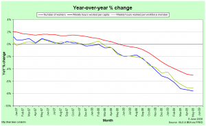
First the year-over-year % change in number of production workers, hours worked per member of the workforce and hours worked per capita:

Year-over-year changes in employment and hours worked

A casual inspection of this graph suggests that the current recession is, for employment, about the same as or a little better than the 1973-75 recession, but that is an incorrect interpretation.  This graph effectively shows rates of change, so it’s not just the depth below zero that matters but the time beneath it as well.  As we will shortly see, the current recession is actually quite a bit worse than the ’73-75 recession and the 2001 recession was a lot worse than it looks.

First, though, it’s instructive to zoom-in to the last year or two on the graph:

Year-over-year change in employment and hours worked (zoomed in)

The red line indicates the year-over-year change in employment.  It’s clearly badly negative.  The green line is the change in hours worked per member of the workforce.  This is worse than that for employment because not only are people losing their jobs, but those who keep their jobs are, on average, having their hours cut.  The blue line is the change in hours worked per capita.  This is the worst of the three because in addition to people losing their jobs and those with jobs having their hours cut, some of those without jobs have given up looking.  Notice that the blue and green lines were pretty close together at first.  This suggests that in the first half of the current recession, people who lost their jobs were staying in the workforce in the hope of finding work, while it was only in the second half that some of the unemployed started to lose hope and give up looking.

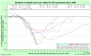
In comparing recessions, I prefer to use the hours-worked-per-capita metric because it captures much more of the employment picture than just employment figures or total hours worked.  Here is a comparison between recessions dating back to 1964, centred around their NBER-determined peak in economic activity:

Comparing hours worked per capita in US recessions relative to NBER-determined peaks in economic activity

Notice that hours worked per capita tend to have been falling for some time before the NBER-determined peak in economic activity.  This is because employment is not the be all and end all of the economy and the dating committee has to take those other elements into account as well.

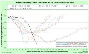
Now we rebase that comparison so each recession is relative to it’s actual peak in hours worked per capita:

Comparing US recessions relative to actual peaks in hours worked per capita

This gives us a true measure of the depth of each recession with respect to employment.  We can see that the ’71-75 and 2001 recessions reached about the same depth and that the current recession has now gone lower than either of them.  Since it is reasonable to assume that the USA will continue to lose jobs (or at least hours worked) in the next couple of months, we can safely call the current recession the worst of this group of seven.

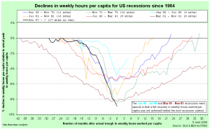
Finally, I thought it worthwhile to compare the falls relative to actual peaks, but centred around each recession’s trough in hours worked per capita (for comparison purposes, I have assumed that the current recession’s trough was in May ’09):

Comparing US recessions in hours worked per capita, centred around their troughs

This graph gives some hope to those imagining a quick recovery.  While the recoveries do tend to be a little slower than the recessions, there does appear to be some symmetry around the troughs.

Is “politician” just another service industry job?

One of my friends disagrees with my thoughts on the MP expenses scandal in Britain.  I’m not entirely sure, but I believe that part of our difference of opinion starts at a disagreement over what it really means to be a politician.

So here is my question to the world at large (yes, I recognise that it might be a false dichotomy): Is “politician” a job title just like any other, or is being a politician to have some sort of sacred, noble trust? Is there is something more to the role than simply maximising the returns to your constituents or the country as a whole?

Let me propose a thought experiment (for any American’s in the audience, parliament = congress and MP = representative).

Suppose we change the law so that a) voting for your representative to parliament is mandatory; b) each member of parliament represents exactly the same number of people; and c) in addition to electing a representative to parliament, everybody is permitted to vote directly on any matter brought before that parliament. If you choose to vote directly on an issue, then the weight of your representative’s vote is decreased proportionately. In this way, we would have the possibility of anything between 100% pure direct democracy and standard representative democracy, depending on what people choose.

How many people would choose to vote directly on some issues? How many on every issue? Clearly the answer is that we’d have a distribution. Some people would vote directly on everything, some would do so occasionally and some never at all.

So what do we make of that distribution? I’ll grant that I’m thinking like an economist here, but I think it’s a perfectly normal, mundane choice between trade-offs. Should I pay attention to the debate on fishing regulation or should I do something else? Everybody faces a different combination of available options, preferences over those options, incomes and relative prices between those options, so any range of attention to parliament might emerge.

In that situation, choosing to not vote directly is entirely equivalent to taking your shirts to the dry cleaner or hiring a maid to clean your house once a week. It’s an economic decision like any other, which in turn makes “politician” just another service industry job title like “financial adviser” or “maid”.

[Side note: This scenario is currently my ideal. If I could, I’d have MPs  paid per parliamentary vote per person represented, with a negative hit to anybody that introduced a bill to parliament so as to discourage frivolous votes.]

Update (1 June ’09): Put another way, why should a backbench opposition MP, who has only an abstract and indirect power over my life, be subject to more stringent ethical standards than the person performing heart surgery on me, who has direct and absolute power over my life?

Counter-cyclical markups

One of the things that gets discussed in the currently-under-attack topic of DSGE models is that of counter-cyclical markups.  If the typical firm’s markup is counter-cyclical — that is, if it’s markup over marginal cost rises during a recession and falls during a boom — then both the magnitude and the duration of any given shock to the economy will be larger.

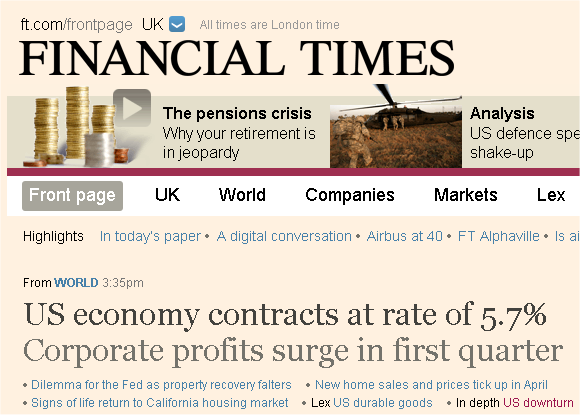
From the front page of the FT website this afternoon:

counter-cyclical profits

The article it’s referring to is here.

Busy

So on top of the financial crisis in general, the bank stress tests in particular, the ensuing recession, the reaching out in foreign policy, the push for healthcare reform, the changes in taxation policy, the regulation of carbon dioxide, the implosion of the US car industry and an influenza pandemic, Obama now gets to deal with a retiring supreme court judge.  And he’s now in day 103 or something.

Is America recapitalising all the non-American banks?

The recent naming of the AIG counterparties [press release, NY Times coverage] reminded me of something and this post by Brad Setser has inspired me to write on it.

Back in January, I wrote a post that contained some mistakes.  I argued that part of the reason that the M1 money multiplier in America fell below unity was because foreign banks with branches in America and American banks with branches in other countries were taking deposits from other countries and placing them in (excess) reserve at the Federal Reserve.

My first mistake was in believing that that was the only reason why the multiplier fell below one.  Of course, even if the United States were in a state of autarky it could still fall below one as all it requires is that banks withdraw from investments outside the standard definitions of money and place the proceeds in their reserve account at the Fed.

And that was certainly happening, because by paying interest on excess reserves, the Fed placed a floor under the risk-adjusted return that banks would insist on receiving for any investment.  Any position with a risk-free-equivalent yield that was less than what the Fed was paying was very rapidly unwound.

Nevertheless, I believe that my idea still applies in part.  By paying interest on excess reserves, the Fed (surely?) also placed a floor under the risk-adjusted returns for anybody with access to a US depository institution, including foreign branches of US banks and foreign banks with branches in America.  The only difference is that those groups would also have had exchange-rate risk to incorporate.  But since the US dollar enjoys reserve currency status, it may have seemed a safe bet to assume that the USD would not fall while the money was in America at the Fed because of the global flight to quality.

The obvious question is to then ask how much money held in (excess) reserve at the Fed originated from outside of America.  Over 2008:Q4, the relevant movements were: [1]

Remember that, roughly speaking, the definitions are:

  • monetary base = currency + required reserves + excess reserves
  • m1 = currency + demand deposits

So we can infer that next to the $707 billion increase in excess reserves, demand deposits only increased by $148 billion and required reserves by $7 billion.

In a second mistake in my January post, I thought that it was the difference in growth between m1 and the monetary base that needed explaining.  That was silly.  Strictly speaking it is the entirety of the excess reserve growth that we want to explain.  How much was from US banks unwinding domestic positions and how much was from foreigners?

Which is where we get to Brad’s post.  In looking at the latest Flow of Funds data from the Federal Reserve, he noted with some puzzlement that over 2008:Q4 for the entire US banking system (see page 69 of the full pdf):

  • liabilities to domestic banks (floats and discrepancies in interbank transactions) went from $-50.9 billion to $-293.4 billion.
  • liabilities to foreign banks went from $-48.1 billion to $289.5 billion

I’m not sure about the first of those, but on the second that represents a net loan of $337.6 billion from foreign banks to US banks over that last quarter.

Could that be foreign banks indirectly making use of the Fed’s interest payments on excess reserves?

No matter what the extent of foreign banks putting money in reserve with the Fed, that process – together with the US government-backed settlements of AIGs foolish CDS contracts – amounts to America (partially) recapitalising not just its own, but the banking systems of the rest of the world too.

[1] M1 averaged 1435.1 in September and 1624.7 in December.  Monetary base averaged 936.138 in September and 1692.511 in December.  Currency averaged 776.7 in September and 819.0 in December. Excess reserves averaged 60.051 in September and 767.412 in December.  Remember that the monthly figures released by the Federal Reserve are dated at the 1st of the month but are actually an average for the whole of the month.

How to value toxic assets (part 5)

John Hempton has an excellent post on valuing the assets on banks’ balance sheets and whether banks are solvent.  He starts with a simple summary of where we are:

We have a lot of pools of bank assets (pools of loans) which have the following properties:
  • The assets sit on the bank’s balance sheet with a value of 90 – meaning they have either being marked down to 90 (say mark to mythical market or model) or they have 10 in provisions for losses against them.
  • The same assets when they run off might actually make 75 – meaning if you run them to maturity or default the bank will – discounted at a low rate – recover 75 cents in the dollar on value.

The banks are thus under-reserved on an “held to maturity” basis. Heavily under-reserved.

He then gives another explanation (on top of the putting-Humpty-Dumpty-back-together-again idea I mentioned previously) of why the market price is so far below the value that comes out of standard asset pricing:

Before you go any further you might wonder why it is possible that loans that will recover 75 trade at 50? Well its sort of obvious – in that I said that they recover 75 if the recoveries are discounted at a low rate. If I am going to buy such a loan I probably want 15% per annum return on equity.

The loan initially yielded say 5%. If I buy it at 50 I get a running yield of 10% – but say 15% of the loans are not actually paying that yield – so my running yield is 8.5%. I will get 75-80c on them in the end – and so there is another 25cents to be made – but that will be booked with an average duration of 5 years – so another 5% per year. At 50 cents in the dollar the yield to maturity on those bad assets is about 15% even though the assets are “bought cheap”. That is not enough for a hedge fund to be really interested – though if they could borrow to buy those assets they might be fun. The only problem is that the funding to buy the assets is either unavailable or if available with nasty covenants and a high price. Essentially the 75/50 difference is an artefact of the crisis and the unavailability of funding.

The difference between the yield to maturity value of a loan and its market value is extremely wide. The difference arises because you can’t eaily borrow to fund the loans – and my yield to maturity value is measured using traditional (low) costs of funds and market values loans based on their actual cost of funds (very high because of the crisis).

The rest of Hempton’s piece speaks about various definitions of solvency, whether (US) banks meet each of those definitions and points out the vagaries of the plan recently put forward by Geithner.  It’s all well worth reading.

One of the other important bits:

Few banks would meet capital adequacy standards. Given the penalty for even appearing as if there was a chance that you would not meet capital adequacy standards is death (see WaMu and Wachovia) and this is a self-assessed exam, banks can be expected not to tell the truth.

(It was Warren Buffett who first – at least to my hearing – described financial accounts as a self-assessed exam for which the penalty for failure is death. I think he was talking about insurance companies – but the idea is the same. Truth is not expected.)

Other posts in this series:  1, 2, 3, 4, [5], 6.

How to value toxic assets (part 4)

Okay.  First, a correction:  There is (of course) a market for CDOs and other such derivatives at the moment.  You can sell them if you want.  It’s just that the prices that buyers are willing to pay is below what the holders of CDOs are willing to accept.

So, here are a few thoughts on estimating the underlying, or “fair,” value of a CDO:

Method 1. Standard asset pricing considers an asset’s value to be the sum of the present discounted value of all future income that it generates.  We discount future income because:

  • Inflation will mean that the money will be worth less in the future, so in terms of purchasing power, we should discount it when thinking of it in today’s terms.
  • Even if there were no inflation, if we got the money today we could invest it elsewhere, so we need to discount future income to allow for the (lost) opportunity cost if current investment options generate a higher return than what the asset is giving us.
  • Even if there were no inflation and no opportunity cost, there is a risk that we won’t receive the future money.  This is the big one when it comes to valuing CDOs and the like.
  • Even if there’s no inflation, no opportunity cost and no risk of not being paid, a positive pure rate of time preference means that we’d still prefer to get our money today.

The discounting due to the risk of non-payment is difficult to quantify because of the opacity of CDOs.  The holders of CDOs don’t know exactly which mortgages are at the base of their particular derivative structure and even if they did, they don’t know the household income of each of those borrowers.  Originally, they simply trusted the ratings agencies, believing that something labeled “AAA” would miss payment with probability p%, something “AA” with probability q% and so on.  Now that the ratings handed out have been shown to be so wildly inappropriate, investors in CDOs are being forced to come up with new numbers.  This is where Knightian Uncertainty is coming into effect:  Since even the risk is uncertain, we are in the Rumsfeldian realm of unknown unknowns.

Of course we do know some things about the risk of non-payment.  It obviously rises as the amount of equity a homeowner has falls and rises especially quickly when they are underwater (a.k.a. have negative equity (a.k.a. they owe more than the property is worth)).  It also obviously rises if there have been a lot of people laid off from their jobs recently (remember that the owner of a CDO can’t see exactly who lies at the base of the structure, so they need to think about the probability that whoever it is just lost their job).

The first of those is the point behind this idea from Chris Carroll out of NYU:  perhaps the US Fed should simply offer insurance against falls in US house prices.

The second of those will be partially addressed in the future by this policy change announced recently by the Federal Housing Finance Agency:

[E]ffective with mortgage applications taken on or after Jan. 1, 2010, Freddie Mac and Fannie Mae are required to obtain loan-level identifiers for the loan originator, loan origination company, field appraiser and supervisory appraiser … With enactment of the S.A.F.E. Mortgage Licensing Act, identifiers will now be available for each individual loan originator.

“This represents a major industry change. Requiring identifiers allows the Enterprises to identify loan originators and appraisers at the loan-level, and to monitor performance and trends of their loans,” said Lockhart [, director of the FHFA].

It’s only for things bought by Fannie and Freddie and it’s only for future loans, but hopefully this will help eventually.

Method 2. The value of different assets will often necessarily covary.  As a absurdly simple example, the values of the AAA-rated and A-rated tranches of a CDO offering must provide upper and lower bounds on the value of the corresponding AA-rated tranche.  Statistical estimation techniques might therefore be used to infer an asset’s value.  This is the work of quantitative analysts, or “quants.”

Of course, this sort of analysis will suffer as the quality of the inputs falls, so if some CDOs have been valued by looking at other CDOs and none of them are currently trading (or the prices of those trades are different to the true values), then the value of this analysis correspondingly falls.

Method 3. Borrowing from Michael Pomerleano’s comment in rely to Christopher Carroll’s piece, one extreme method of valuing CDOs is to ask at what price a distressed debt (a.k.a. vulture) fund would be willing to buy them at with the intention of merging all the CDOs and other MBSs for a given mortgage pool so that they could then renegotiate the debt with the underlying borrowers (the people who took out the mortgages in the first place).  This is, in essense, a job of putting Humpty Dumpty back together again.  Gathering all the CDOs and other MBSs for a given pool of mortgage assets will take time.  Identifying precisely those mortgage assets will also take time.  There will be sizable legal costs.  Some holders of the lower-rated CDOs may also refuse to sell if they realise what’s happening, hoping to draw out some rent extraction from the fund.  The price that the vulture fund would offer on even the “highly” rated CDOs would therefore be very low in order to ensure that they made a profit.

It would appear that banks and other holders of CDOs and the like are using some combination of methods one and two to value their assets, while the bid-prices being offered by buyers are being set by the logic of something like method three.  Presumably then, if we knew the banks’ private valuations, we might regard the difference between them and the market prices as the value of the uncertainty.

Other posts in this series:  1, 2, 3, [4], 5, 6.
One of the challenges in negotiation for Israel/Palestine

There’s a perennial idea of proposing Northern Ireland as a model of how progress might be achieved in the fighting between Israelis and Palestinians.  After reading this recent posting by Megan McArdle, one of the difficulties in such an idea becomes plain.

In Northern Ireland, both sides had moral, if not logistical, support from larger powers that were themselves allies.  So while the nationalists found it difficult to trust the British government, they would generally trust the US government, who in turn trusted the British government, while the same chain applied in reverse for the loyalists.

By contrast, while Israel receives moral and logistical support from the USA, none of America’s close allies really comes close to giving the Palestinian cause at large, let alone Hamas in particular, the sort of tacit support that America gave the Irish nationalists.

How to value toxic assets (part 3)

Continuing on from my previous thoughts (1, 2, 3, 4) …

In the world of accounting, the relevant phrase here is “fair value.”  In the United States (which presently uses a different set of accounting requirements to the rest of the world, although that is changing), assets are classified as being in one of three levels (I’m largely reproducing the Wikipedia article here):

Level one assets are those traded in liquid markets with quoted prices.  Fair value (in a mark-to-market sense) is taken to be the current price.

Level two and level three assets are not traded in liquid markets with quoted prices, so their fair values need to be estimated via a statistical model.

Level two assets are those whose fair value is able to be estimated by looking at publicly-available market information.  As a contrived example, maybe there is currently no market for a particular AA-rated tranche of CDOs, but there are recent prices for the corresponding AAA-rated and A-rated tranches, so the AA-rated stuff should be valued somewhere in between those two.

Level three assets are those whose fair value can only be estimated by appealing to information that is not publicly observable.

These are listed in the U.S. Financial Accounting Standards Board (FASB) Statement 157.  In October of last year, the FASB issued some clarification/guidance on valuing derivatives like CDOs when the market for them had dried up.

Brad DeLong, in early December last year, was given a list of reasons from Steve Ross why we might not want to always mark-to-market (i.e. assume that the fair value is the currently available market price):

  • If you believe in organizational capital–in goodwill–in the value of the enterprise’s skills, knowledge, and relationships as a source of future cash flows–than marking it to market as if that organizational capital had no value is the wrong thing to do.
    • Especially as times in which asset values are disturbed and impaired are likely to be times when the value of that organizational capital is highest.
  • If you believe in mean reversion in risk-adjusted asset values, mark-to-market accounting is the wrong thing to do.
  • If you believe that transaction prices differ from risk-adjusted asset values–perhaps because transaction prices are of particular assets that are or are feared to be adversely selected and hence are not representative of the asset class–than mark-to-market accounting is the wrong thing to do.
  • If you believe that changes in risk-adjusted asset values are unpredictable, but also believe:
    • in time-varying required expected returns do to changing risk premia;
    • that an entity’s own cost of capital does not necessarily move one-for-one with the market’s time-varying risk premia;
    • then mark-to-market accounting is the wrong thing to do.

Other posts in this series:  1, 2, [3], 4, 5, 6.