The contradictory joys of being the US Treasury Secretary (part 2)

In my last post, I highlighted the apparent contradictions between the USA having both a “strong dollar” policy and a desire to correct their trade deficit (“re-balancing”).  Tim Geithner, speaking recently in Tokyo, declared that there was no contradiction:

Geithner said U.S. efforts to boost exports aren’t in conflict with the “strong-dollar” policy. “I don’t think there’s any contradiction between the policies,” he said.

I then said:

The only way to reconcile what Geithner’s saying with the laws of mathematics is to suppose that his “strong dollar” statements are political and relate only to the nominal exchange rate and observe that trade is driven by the real exchange rate. But that then means that he’s calling for a stable nominal exchange rate combined with either deflation in the USA or inflation in other countries.

Which, together with Nouriel Roubini’s recent observation that the US holding their interest rates at zero is fueling “the mother of all carry trades” [Financial Times, RGE Monitor], provides for a delicious (but probably untrue) sort-of-conspiracy theory:

Suppose that Tim Geithner firmly believes in the need for re-balancing.  He’d ideally like US exports to rise while imports stayed flat (since that would imply strong global growth and new jobs for his boss’s constituents), but he’d settle for US imports falling.  Either way, he needs the US real exchange rate to fall, but he doesn’t care how.  Well, not quite.  His friend Ben Bernanke tells him that he doesn’t want deflation in America, but he doesn’t really care between the nominal exchange rate falling and foreign prices rising (foreign inflation).

The recession-induced interest rates of (effectively) zero in America are now his friend, because he’s going to get what he wants no matter what, thanks to the carry trade.  Private investors are borrowing money at 0% interest in America and then going to foreign countries to invest it at interest rates that are significantly higher than zero.  If the foreign central banks did nothing, that would push the US dollar lower and their own currencies higher and Tim gets what he wants.

But the foreign central banks want a strong dollar because (a) they’re holding gazzilions of dollars worth of US treasuries and they don’t want their value to fall; and (b) they’re not fully independent of their political masters who want to want to keep exporting.   So Tim regularly stands up in public and says that he supports a strong dollar.  That makes him look innocent and excuses the foreign central banks for doing what they were all doing anyway:  printing local money to give to the US-funded investors so as to keep their currencies down (and the US dollar up).

But that means that the money supply in foreign countries is climbing, fast, and while prices may be sticky in the short term, they will start rising soon enough.  Foreign inflation will lower the US real exchange rate and Tim still gets what he wants.

The only hope for the foreign central banks is that the demand for their currencies is a short-lived temporary blip.  In that case, defending their currencies won’t require the creation of too much local currency and they could probably reverse the situation fast enough afterward that they don’t get bad inflation. [This is one of the arguments in favour of central bank involvement in the exchange-rate market.  Since price movements are sluggish, they can sterilise a temporary spike and gradually back out the action before local prices react too much.]

But as foreign central banks have been discovering [1], free money is free money and the carry trade won’t go away until the interest rate gap is sufficiently closed:

Nov. 13 (Bloomberg) — Brazil, South Korea and Russia are losing the battle among developing nations to reduce gains in their currencies and keep exports competitive as the demand for their financial assets, driven by the slumping dollar, is proving more than central banks can handle.

South Korea Deputy Finance Minister Shin Je Yoon said yesterday the country will leave the level of its currency to market forces after adding about $63 billion to its foreign exchange reserves this year to slow the appreciation of the won.
[…]
Brazil’s real is up 1.1 percent against the dollar this month, even after imposing a tax in October on foreign stock and bond investments and increasing foreign reserves by $9.5 billion in October in an effort to curb the currency’s appreciation. The real has risen 33 percent this year.
[…]
“I hear a lot of noise reflecting the government’s discomfort with the exchange rate, but it is hard to fight this,” said Rodrigo Azevedo, the monetary policy director of Brazil’s central bank from 2004 to 2007. “There is very little Brazil can do.”

The central banks are stuck.  They can’t lower their own interest rates to zero (which would stop the carry trade) as that would stick a rocket under domestic production and cause inflation anyway.  The only thing they can do is what Brazil did a little bit of:  impose legal limits on capital inflows, either explicitly or by taxing foreign-owned investments.  But doing that isn’t really an option, either, because they want to be able to keep attracting foreign investment after all this is over and there’s not much scarier to an investor than political uncertainty.

So they have to wait until America raises it’s own rates.  But that won’t happen until America sees a turn-around in jobs and the fastest way for that to happen is for US exports to rise.

[1] Personally, I think the central bankers saw the writing on the wall the minute the Fed lowered US interest rates to (effectively) zero but their political masters were always going to take some time to cotton on.

The contradictory joys of being the US Treasury Secretary

Tim Geithner, speaking at the start of the G-20 meeting in Pittsburgh:

Sept. 25 (Bloomberg) — Treasury Secretary Timothy Geithner said he sees a “strong consensus” among Group of 20 nations to reduce reliance on exports for growth and defended the dollar’s role as the world’s reserve currency.

“A strong dollar is very important in the United States,” Geithner said in response to a question at a press conference yesterday in Pittsburgh, where G-20 leaders began two days of talks.

Tim Geithner, speaking in Tokyo while joining the US President on a tour of Asian capitals:

Nov. 11 (Bloomberg) — U.S. Treasury Secretary Timothy Geithner said a strong dollar is in the nation’s interest and the government recognizes the importance it plays in the global financial system.

“I believe deeply that it’s very important to the United States, to the economic health of the United States, that we maintain a strong dollar,” Geithner told reporters in Tokyo today.
[…]
Geithner said U.S. efforts to boost exports aren’t in conflict with the “strong-dollar” policy. “I don’t think there’s any contradiction between the policies,” he said.

Which is hilarious.

There is no objective standard for currency strength [1].  A “strong (US) dollar” is a dollar strong relative to other currencies, so it’s equivalent to saying “weak non-US-dollar currencies”.  But when the US dollar is up and other currencies are down, that means that the US will import more (and export less), while the other countries will export more (and import less), which is the exact opposite of the re-balancing efforts.

The only way to reconcile what Geithner’s saying with the laws of mathematics is to suppose that his “strong dollar” statements are political and relate only to the nominal exchange rate and observe that trade is driven by the real exchange rate.  But that then means that he’s calling for a stable nominal exchange rate combined with either deflation in the USA or inflation in other countries.

Assuming my previous paragraph is true, 10 points to the person who can see the potential conspiracy theory [2] implication of Nouriel Roubini’s recent observation that the US holding their interest rates at zero is fueling “the mother of all carry trades” [Financial Times, RGE Monitor].

Hint:  If you go for the conspiracy theory, this story would make you think it was working.

Nov. 13 (Bloomberg) — Brazil, South Korea and Russia are losing the battle among developing nations to reduce gains in their currencies and keep exports competitive as the demand for their financial assets, driven by the slumping dollar, is proving more than central banks can handle.
[…]
Governments are amassing record foreign-exchange reserves as they direct central banks to buy dollars in an attempt to stem the greenback’s slide and keep their currencies from appreciating too fast and making their exports too expensive.
[…]
“It looked for a while like the Bank of Korea was trying to defend 1,200, but it looks like they’ve given up and are just trying to slow the advance,” said Collin Crownover, head of currency management in London at State Street Global Advisors

The answer to follow …

Update: The answer is in my next post.

[1] There better not be any gold bugs in the audience.  Don’t make me come over there and hurt you.

[2] Okay, not a conspiracy theory; just a behind-the-scenes-while-completely-in-the-open strategy of international power struggles.

[1] There better not be any gold bugs on this list.  Don’t make me
come over there and hurt you.

[2] Okay, not a conspiracy theory; just a behind-the-scenes-while-
completely-in-the-open strategy of international power struggles.

Not raising the minimum wage with inflation will make your country fat

Via Greg Mankiw, here is a new working paper by David O. Meltzer and Zhuo Chen: “The Impact of Minimum Wage Rates on Body Weight in the United States“. The abstract:

Growing consumption of increasingly less expensive food, and especially “fast food”, has been cited as a potential cause of increasing rate of obesity in the United States over the past several decades. Because the real minimum wage in the United States has declined by as much as half over 1968-2007 and because minimum wage labor is a major contributor to the cost of food away from home we hypothesized that changes in the minimum wage would be associated with changes in bodyweight over this period. To examine this, we use data from the Behavioral Risk Factor Surveillance System from 1984-2006 to test whether variation in the real minimum wage was associated with changes in body mass index (BMI). We also examine whether this association varied by gender, education and income, and used quantile regression to test whether the association varied over the BMI distribution. We also estimate the fraction of the increase in BMI since 1970 attributable to minimum wage declines. We find that a $1 decrease in the real minimum wage was associated with a 0.06 increase in BMI. This relationship was significant across gender and income groups and largest among the highest percentiles of the BMI distribution. Real minimum wage decreases can explain 10% of the change in BMI since 1970. We conclude that the declining real minimum wage rates has contributed to the increasing rate of overweight and obesity in the United States. Studies to clarify the mechanism by which minimum wages may affect obesity might help determine appropriate policy responses.

Emphasis is mine.  There is an obvious candidate for the mechanism:

  1. Minimum wages, in real terms, have been falling in the USA over the last 40 years.
  2. Minimum-wage labour is a significant proportion of the cost of “food away from home” (often, but not just including, fast-food).
  3. Therefore the real cost of producing “food away from home” has fallen.
  4. Therefore the relative price of “food away from home” has fallen.
  5. Therefore people eat “food away from home” more frequently and “food at home” less frequently.
  6. Typical “food away from home” has, at the least, more calories than “food at home”.
  7. Therefore, holding the amount of exercise constant,  obesity rates increased.

Update: The magnitude of the effect for items 2) – 7) will probably be greater for fast-food versus regular restaurant food, because minimum-wage labour will almost certainly comprise a larger fraction of costs for a fast-food outlet than it will for a fancy restaurant.

Variation in US unemployment

The NY Times brings us a another wonderful graphic.  As of September 2009, white women aged 25 to 34 with a college degree had an unemployment rate of just 3.6%, while black men aged 18 to 24 without a highschool diploma had an unemployment rate of 48.5%.  Change that last group to white men aged 18 to 24 without a highschool diploma and it falls to 25.6%.

The likelihood-ratio threshold is the shadow price of statistical power

Cosma Shalizi, an associate professor in statistics at Carnegie Mellon University, gives an interpretation of the likelihood-ratio threshold in an LR test: It’s the shadow price of statistical power:

[…]

Suppose we know the probability density of the noise p and that of the signal is q. The Neyman-Pearson lemma, as many though not all schoolchildren know, says that then, among all tests off a given size s, the one with the smallest miss probability, or highest power, has the form “say ‘signal’ if q(x)/p(x) > t(s), otherwise say ‘noise’,” and that the threshold t varies inversely with s. The quantity q(x)/p(x) is the likelihood ratio; the Neyman-Pearson lemma says that to maximize power, we should say “signal” if its sufficiently more likely than noise.

The likelihood ratio indicates how different the two distributions — the two hypotheses — are at x, the data-point we observed. It makes sense that the outcome of the hypothesis test should depend on this sort of discrepancy between the hypotheses. But why the ratio, rather than, say, the difference q(x) – p(x), or a signed squared difference, etc.? Can we make this intuitive?

Start with the fact that we have an optimization problem under a constraint. Call the region where we proclaim “signal” R. We want to maximize its probability when we are seeing a signal, Q(R), while constraining the false-alarm probability, P(R) = s. Lagrange tells us that the way to do this is to minimize Q(R) – t[P(R) – s] over R and t jointly. So far the usual story; the next turn is usually “as you remember from the calculus of variations…”

Rather than actually doing math, let’s think like economists. Picking the set R gives us a certain benefit, in the form of the power Q(R), and a cost, tP(R). (The ts term is the same for all R.) Economists, of course, tell us to equate marginal costs and benefits. What is the marginal benefit of expanding R to include a small neighborhood around the point x? Just, by the definition of “probability density”, q(x). The marginal cost is likewise tp(x). We should include x in R if q(x) > tp(x), or q(x)/p(x) > t. The boundary of R is where marginal benefit equals marginal cost, and that is why we need the likelihood ratio and not the likelihood difference, or anything else. (Except for a monotone transformation of the ratio, e.g. the log ratio.) The likelihood ratio threshold t is, in fact, the shadow price of statistical power.

It seems sensible to me.

Who has more information, the Central Bank or the Private Sector?

A friend pointed me to this paper:

Svensson, Lars E. O. and Michael Woodford. “Indicator Variables For Optimal Policy,” Journal of Monetary Economics, 2003, v50(3,Apr), 691-720.

You can get the NBER working paper (w8255) here.  The abstract:

The optimal weights on indicators in models with partial information about the state of the economy and forward-looking variables are derived and interpreted, both for equilibria under discretion and under commitment. The private sector is assumed to have information about the state of the economy that the policymaker does not possess. Certainty-equivalence is shown to apply, in the sense that optimal policy reactions to optimally estimated states of the economy are independent of the degree of uncertainty. The usual separation principle does not hold, since the estimation of the state of the economy is not independent of optimization and is in general quite complex. We present a general characterization of optimal filtering and control in settings of this kind, and discuss an application of our methods to the problem of the optimal use of ‘real-time’ macroeconomic data in the conduct of monetary policy. [Emphasis added by John Barrdear]

The sentence I’ve highlighted is interesting.  As written in the abstract, it’s probably true.  Here’s a paragraph from page two that expands the thought:

One may or may not believe that central banks typically possess less information about the state of the economy than does the private sector. However, there is at least one important argument for the appeal of this assumption. This is that it is the only case in which it is intellectually coherent to assume a common information set for all members of the private sector, so that the model’s equations can be expressed in terms of aggregative equations that refer to only a single “private sector information set,” while at the same time these model equations are treated as structural, and hence invariant under the alternative policies that are considered in the central bank’s optimization problem. It does not make sense that any state variables should matter for the determination of economically relevant quantities (that is, relevant to the central bank’s objectives), if they are not known to anyone in the private sector. But if all private agents are to have a common information set, they must then have full information about the relevant state variables. It does not follow from this reasoning, of course, that it is more accurate to assume that all private agents have superior information to that of the central bank; it follows only that this case is one in which the complications resulting from partial information are especially tractable. The development of methods for characterizing optimal policy when di fferent private agents have di fferent information sets remains an important topic for further research.

Here’s my attempt as paraphrasing Svensson and Woodford in point form:

  1. The real economy is the sum of private agents (plus the government, but ignore that)
  2. Complete information is thus, by definition, knowledge of every individual agent
  3. If we assume that everybody knows about themselves (at least), then the union of all private information sets must equal complete information
  4. The Central Bank observes only a sample of private agents
  5. That is, the Central Bank information set is a subset of the union of all private information sets. The Central Bank’s information cannot be greater than the union of all private information sets.
  6. One strategy in simplifying the Central Bank’s problem is to assume that private agents are symmetric in information (i.e. they have a common information set).  In that case, we’d say that the Central Bank cannot have more information than the representative private sector agent. [See note 1 below]
  7. Important future research will involve relaxing the assumption in (f) and instead allowing asymmetric information across different private agents.  In that world, the Central Bank might have more information than any given private agent, but still less than the union of all private agents.

Svensson and Woodford then go on to consider a world where the Central Bank’s information set is smaller than (i.e. is a subset of) the Private Sector’s common information set.

But that doesn’t really make sense to me.

If private agents share a common information set, it seems silly to suppose that the Central Bank has less information than the Private Sector, for the simple reason that the mechanism of creating the common information set – commonly observable prices that are sufficient statistics of private signals – is also available to the Central Bank.

In that situation, it seems more plausible to me to argue that the CB has more information than the Private Sector, provided that their staff aren’t quietly acting on the information on the side.  It also would result in observed history:  the Private Sector pays ridiculous amounts of attention to every word uttered by the Central Bank (because the Central Bank has the one private signal that isn’t assimilated into the price).

Note 1: To arrive at all private agents sharing a common information set, you require something like the EMH (in fact, I can’t think how you could get there without the EMH).  A common information set emerges from a commonly observable sufficient statistic of all private information.  Prices are that statistic.

    The death throes of US newspapers?

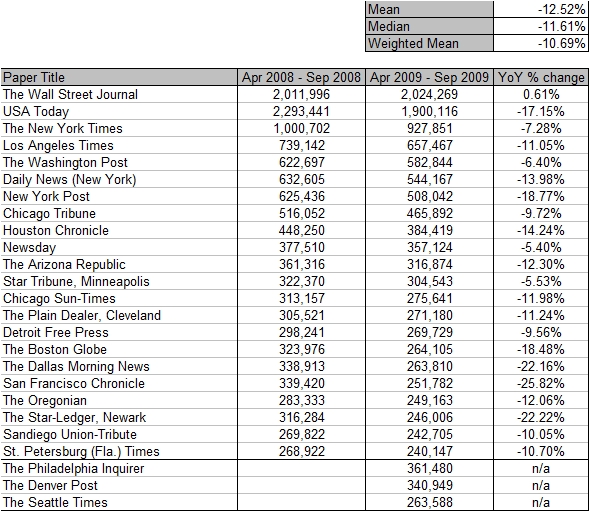
    Via Megan McArdle’s excellent commentary, I discovered the Mon-Fri daily circulation figures for the top 25 newspapers in the USA.  Megan’s words:

    I think we’re witnessing the end of the newspaper business, full stop, not the end of the newspaper business as we know it. The economics just aren’t there. At some point, industries enter a death spiral: too few consumers raises their average costs, meaning they eventually have to pass price increases onto their customers. That drives more customers away. Rinse and repeat . . .

    […]

    The numbers seem to confirm something I’ve thought for a while: we’re eventually going to end up with a few national papers, a la Britain, rather than local dailies. The Wall Street Journal, the Washington Post, and the New York Times (sorry, conservatives!) are weathering the downturn better than most, and it’s not surprising: business, politics, and national upper-middlebrow culture. But in 25 years, will any of them still be printing their product on the pulped up remains of dead trees? It doesn’t seem all that likely.

    For those of you that like your information in pictoral form, here it is:

    First, the data.  Look at the Mean/Median/Weighted Mean figures.  That really is an horrific collapse in sales.

    US_Newspaper_circulation_data

    Second, the distribution (click on the image for a full-sized version):

    US_Newspaper_circulation_distribution

    Finally, a scatter plot of year-over-year change against the latest circulation figures (click on the image for a full-sized version):

    US_Newspaper_circulation_scatterplotAs Megan alluded in the second paragraph I quoted, there appears to be a weak relationship between the size of the paper and the declines they’ve suffered, with the bigger papers holding up better.  The USA Today is the clear exception to that idea.  Indeed, if the USA Today is excluded from the (already very small!) sample the R^2 becomes 30%.

    To really appreciate just how devestating those numbers are, you need to combine it with advertising figures.  Since newspapers take revenue from both sales (circulation) and advertising, the fact that advertising revenue has also collapsed, as it always does in a recession, means that newspapers have taken not just one but two knives to the chest.

    Here’s advertising expenditure in newspapers over recent years, taken from here:

    Year Expenditure (millions of dollars) Year-over-year % change
    2005 47,408
    2006 46,611 -1.7%
    2007 42,209 -9.2%
    2008 34,740 -17.7%

    Which is ugly.  Remember, also, that this expenditure is nominal.  Adjusted for inflation, the figures will be worse.

    So what do you do when your ad sales and your circulation figures both fall by over 15%?  Oh, and you can’t really cut costs any more because, as Megan says:

    For twenty years, newspapers have been trying to slow the process with increasingly desperate cost cutting, but almost all are at the end of that rope; they can’t cut their newsroom or production staff any further and still put out a newspaper. There just aren’t enough customers who are willing to pay for their product what it costs to produce it.

    Which, in economics speak, means that the newspaper business has a large fixed cost component that isn’t particularly variable even in the long run.

    Tyler Cowen, in an excellent post that demonstrates precisely why I read him daily, says:

    I believe with p = 0.6 that the world is in for a “great disruption.”  It has come to MSM first but it will not end there.  In the longer run I am optimistic about the results of this change — computers will free up lots of human labor — but in the meantime it will have drastic implications for income redistribution, across both individuals and across economic sectors.  For a core metaphor, the internet displacing paid journalism and classified ads is a good place to start.  The value of newspapers has been sucked into Google.

    […]Once The Great Disruption becomes more evident, entertainment will be very very cheap.

    Which may well be true, but will be cold comfort for all of those traditional journalists out there.

    Be careful interpreting Lagrangian multipliers

    Last year I wrote up a derivation of the New Keynesian Phillips Curve using Calvo pricing.  At the start of it, I provided the standard pathway from the Dixit-Stiglitz aggregator for consumption to the constant own-price elasticity individual demand function.  Let me reproduce it here:

    There is a constant and common elasticity of substitution between each good: $$\varepsilon>1$$.  We aggregate across the different consumptions goods:

    $$!C=\left(\int_{0}^{1}C\left(i\right)^{\frac{\varepsilon-1}{\varepsilon}}di\right)^{\frac{\varepsilon}{\varepsilon-1}}$$

    $$P\left(i\right)$$ is the price of good i, so the total expenditure on consumption is $$\int_{0}^{1}P\left(i\right)C\left(i\right)di$$

    A representative consumer seeks to minimise their expenditure subject to achieving at least $$C$$ units of aggregate consumption. Using the Lagrange multiplier method:

    $$!L=\int_{0}^{1}P\left(i\right)C\left(i\right)di-\lambda\left(\left(\int_{0}^{1}C\left(i\right)^{\frac{\varepsilon-1}{\varepsilon}}di\right)^{\frac{\varepsilon}{\varepsilon-1}}-C\right)$$

    The first-order conditions are that, for every intermediate good, the first derivative of $$L$$ with respect to $$C\left(i\right)$$ must equal zero. This implies that:

    $$!P\left(i\right)=\lambda C\left(i\right)^{\frac{-1}{\varepsilon}}\left(\int_{0}^{1}C\left(j\right)^{\frac{\varepsilon-1}{\varepsilon}}dj\right)^{\frac{1}{\varepsilon-1}}$$

    Substituting back in our definition of aggregate consumption, replacing $$\lambda$$ with $$P$$ (since $$\lambda$$ represents the cost of buying an extra unit of the aggregate good $$C$$) and rearranging, we end up with the demand curve for each intermediate good:

    $$!C\left(i\right)=\left(\frac{P\left(i\right)}{P}\right)^{-\varepsilon}C$$

    If that Lagrangian looks odd to you, or if you’re asking where the utility function’s gone, you’re not alone.  It’s obviously just the dual problems of consumer theory – the fact that it doesn’t matter if you maximise utility subject to a budget constraint or minimise expenditure subject to a minimum level of utility – but what I want to focus on is the resulting interpretation of the lagrangian multipliers.

    Let’s rephrase the problem as maximising utility, with utility a generic function of aggregate consumption, $$U\left(C\right)$$.  The Lagrangian is then:

    $$!L=U\left(\left(\int_{0}^{1}C\left(i\right)^{\frac{\varepsilon-1}{\varepsilon}}di\right)^{\frac{\varepsilon}{\varepsilon-1}}\right)+\mu\left(M-\int_{0}^{1}P\left(i\right)C\left(i\right)di\right)$$

    The first-order conditions are:

    $$!U’\left(C\right)\left(\int_{0}^{1}C\left(j\right)^{\frac{\varepsilon-1}{\varepsilon}}dj\right)^{\frac{1}{\varepsilon-1}}C\left(i\right)^{\frac{-1}{\varepsilon}}=\mu P\left(i\right)$$

    Rearranging and substituting back in the definition for $$C$$ then gives us:

    $$!C\left(i\right)=\left(P\left(i\right)\frac{\mu}{U’\left(C\right)}\right)^{-\varepsilon}C$$

    In the first approach, $$\lambda$$ represents the cost of buying an extra unit of the aggregate good $$C$$, which is the definition of the aggregate price level.  In the second approach, $$\mu$$ represents the cost of buying an extra unit of income, which is not the same thing.  Comparing the two results, we can see that:

    $$!\lambda=P=\frac{U’\left(C\right)}{\mu}$$

    Which should cause you to raise an eyebrow.  Why aren’t the two multipliers just the inverses of each other?  Aren’t they meant to be?  Yes, they are, but only when the two problems are equivalent.  These two problems are slightly different.

    In the first one, to be equivalent, the term in the lagrangian would need to be $$V – U\left(\left(\int_{0}^{1}C\left(i\right)^{\frac{\varepsilon-1}{\varepsilon}}di\right)^{\frac{\varepsilon}{\varepsilon-1}}\right)$$, which would give us Hicksian demands as a function of utility level ($$V$$).  But since we assumed that utility is only a function of aggregate consumption, then in order to pin down a level of utility, it’s sufficient to pin down a level of aggregate consumption; and that is useful to us because a) a level of utility doesn’t mean much to us as macroeconomists but a level of aggregate consumption does and b) it means that we can recognise the lagrange multiplier as the aggregate price level.

    Which, when you think about it, makes perfect sense.  Extra income must be adjusted by the marginal value of the extra consumption it affords in order to arrive at the price that the (representative) consumer would be willing to pay for that consumption.

    In other words:  be careful when interpreting your Lagrangian multipliers.

    Regulation should set information free

    Imagine that you’re a manager for a large investment fund and you’ve recently been contemplating your position on Citigroup.  How would this press release from Citi affect your opinion of their prospects?:

    New York – Citi today announced the sale of its entire ownership interest of three North American partner credit card portfolios representing approximately $1.3 billion in managed assets. The cards portfolios were part of Citi Holdings. Terms of the deals were not disclosed. Citi will continue to service the portfolios through the first half of 2010 at which time the acquirer will assume all customer servicing aspects of the portfolios.

    The sale of these card portfolios is consistent with Citi’s strategy to optimize the assets and businesses within Citi Holdings while working to generate long-term profitability and growth from Citicorp, which comprises its core franchise. Citi continues to make progress on its strategy and will continue to pursue opportunities within Citi Holdings that create the most value for stakeholders.

    The answer should be “not much, or perhaps a little negatively” because the press release contains close to no information at all.  Here is Floyd Norris:

    A few unanswered questions:

    1. Who is the buyer?
    2. Which card portfolios are being sold?
    3. What is the price?
    4. Is there a profit or loss?

    A check of Citi’s last set of disclosures shows that Citi Holdings had $67.6 billion in such credit card portfolios in the second quarter, so this is a small part of that. Still, I can’t remember a deal announcement when a company said it had sold undisclosed assets to an undisclosed buyer for an undisclosed price, resulting in an undisclosed profit or loss.

    Chris Kaufman at Reuters noted the same.

    Now, to be fair, there is some information in the release if you have some context.  In January 2009 Citigroup separated “into Citicorp, housing its key banking business, and Citi Holdings, which included its brokerage, consumer finance, and troubled assets.”  In other words, Citi Holdings is the bucket holding “assets that Citigroup is trying to sell or wind down.”  The press release is a signal to the market that Citi has been able to offload some of those assets – it’s an attempt to speak of improved market conditions.  But the refusal to release any details suggests that they sold the portfolios at a deep discount to face value, which implies either that Citi was desperate for the cash (a negative signal) or that they think the portfolios were worth even less than they got for them, which doesn’t bode well for the rest of their credit card holdings (also a negative signal).  It’s unsurprising, then, that Citi were down 4.1% in afternoon trading after the release.

    Some more information did emerge later on.  American Banker, citing “industry members with knowledge of the transaction,” reported:

    The buyer was U.S. Bancorp, according to industry members with knowledge of the transaction, who identified the assets as the card portfolios for KeyCorp and Associated Banc-Corp, which Citi issues as an agent bank, and the affinity card for the American Dental Association.

    But a spokeswoman for Citi, which only identified the portfolios as “North American partner credit card portfolios” in a press release, would not comment, identify the buyer, or elaborate on the release. U.S. Bancorp, Associated Bank and the American Dental Association did not return calls by press time; a spokesman for KeyCorp would not discuss the matter.

    It’s tremendously frustrating that even this titbit of information needed to be extracted via a leak.  Did Maria Aspan — the author of the piece at American Banker — take somebody out for a beer?  Did the information come from somebody at Citigroup, Bancorp or one of the law firms that represent them?

    In what seems perfectly designed to turn that furstration into anger, we then have other media outlets reporting this extra information unattributedHere‘s the Wall Street Journal:

    Citigroup Inc. sold its interest in three North American credit-card portfolios to U.S. Bancorp of Minneapolis, continuing the New York bank’s effort to unload assets that aren’t considered to be a core part of its business, according to people familiar with the situation.

    […]

    Citigroup announced the sale, but it didn’t identify the buyer or type of portfolio that was being sold. Representatives of U.S. Bancorp couldn’t be reached for comment.

    That’s it.  There’s no mention of where they got Bancorp from at all.

    It’s all whispers and rumours, friendships and acquaintences.  It’s no way for the market to get their information.

    Here’s my it’ll-never-happen suggestion for improving banking regulation:

    Any purchase or sale of assets representing more than 1% of a bank’s previous holdings in that asset class [in this case the sale represented 1.9% of Citi’s credit card holdings] must be accompanied by the immediate public release of information uniquely identifing the assets bought or sold and the agreed terms of the deal, including the price.  Identities of all parties involved must be publicly disclosed within 6 months of the transaction.