Negative productivity shocks are conceptually okay when applied idiosyncratically to labour

This is mostly a note to myself.

Way back in the dawn of the modern-macro era, the fresh-water Chicago kids came up with Real Business Cycle theory where they endogenised the labour supply and claimed that macro variation was explained by productivity shocks.

The salt-water gang then accepted the techniques of RBC but proposed a bunch of demand-side shocks instead.

The big criticism of productivity shocks has always been to ask how you can realistically get negative shocks to productivity.  Technological regress just doesn’t seem all that likely.

Now, models of credit cycles like Kiotaki (1998) show how a small and temporary negative shock to productivity can turn into a large and persistent downturn in the economy.  In short:  Credit constraints mean that some wealth remains in the hands of the unproductive instead of being lent to the productive sectors of the economy.  The share of wealth owned by the productive is therefore a factor in aggregate output.  A temporary negative shock to productivity keeps more of the wealth with the unproductive for production purposes and it takes time for the productive sector to accumulate its wealth back.  If some sort of physical capital (e.g. land) is used as collateral, the shock will also lower the price of the capital, thus decreasing the value of the collateral and so imposing tighter restrictions on credit.

But Kiyotaki’s model still requires some productive regress …

Looking at Aiyagari (1994) and Castaneda, Diaz-Gimenez and Rios-Rull (2003) today (lecture 3 by Michaelides in EC442), I realise that small negative productivity shocks are conceptually okay if they’re applied idiosyncratically (i.e. individually) to labour.

Let s_{t} be your efficiency state in period ts is a Markov process with transition matrix \Gamma_{ss}e\left(s\right) is the efficiency of somebody in state s.  Castaneda, Diaz-Gimenez and Rios-Rull use this calibration, taken from the data:

State s=1 s=2 s=3 s=4
e(s) 1.00 3.15 9.78 1,061.00
Share of population 61.1% 22.35% 16.50% 0.05%

The transition matrix would be such that the population-shares for each state are stationary.

A household’s labour income is then given by e(s)wl.

A movement from s=3 to s=2, say, is therefore a negative labour productivity shock for the household.

The trick is to think of the efficiency states as job positions. Somebody moving from s=3 to s=1 is losing their job as an engineer and getting a job as an office cleaner.  They will probably increase l to partially compensate for the lose in hourly wage (e\left(s\right)w).

Remember that in the (Neo/New) Classical models, there’s an assumption of zero unemployment.  However much you want to work, that’s how much you work.  [That might sound silly to a casual reader, but it’s okay as a first approximation.  There are (i.e. search-and-matching) models out there that look at unemployment and can be fitted into this framework.]

If everybody is equally good at every job position (as we have here) and all the idiosyncratic shocks balance out so the population shares are constant, then – I believe – there shouldn’t be any change in observed aggregate productivity.

However, if you introduced imperfect transfer of ability across positions so that efficiency becomes e\left(s,\theta\left(s\right)\right) where \theta\left(s\right) is your private type per job position, then idiosyncratic shocks could therefore show up in aggregate numbers.
This is essentially an idea of mismatching.  A senior engineering job is destroyed and a draftsman job is created both in Detroit, while the opposite occurs in Washington state.  Since the engineer in Detroit can’t easily move to Washington, he takes the lower-productivity job and a sub-optimal person gets promoted in Washington.

Is America recapitalising all the non-American banks?

The recent naming of the AIG counterparties [press release, NY Times coverage] reminded me of something and this post by Brad Setser has inspired me to write on it.

Back in January, I wrote a post that contained some mistakes.  I argued that part of the reason that the M1 money multiplier in America fell below unity was because foreign banks with branches in America and American banks with branches in other countries were taking deposits from other countries and placing them in (excess) reserve at the Federal Reserve.

My first mistake was in believing that that was the only reason why the multiplier fell below one.  Of course, even if the United States were in a state of autarky it could still fall below one as all it requires is that banks withdraw from investments outside the standard definitions of money and place the proceeds in their reserve account at the Fed.

And that was certainly happening, because by paying interest on excess reserves, the Fed placed a floor under the risk-adjusted return that banks would insist on receiving for any investment.  Any position with a risk-free-equivalent yield that was less than what the Fed was paying was very rapidly unwound.

Nevertheless, I believe that my idea still applies in part.  By paying interest on excess reserves, the Fed (surely?) also placed a floor under the risk-adjusted returns for anybody with access to a US depository institution, including foreign branches of US banks and foreign banks with branches in America.  The only difference is that those groups would also have had exchange-rate risk to incorporate.  But since the US dollar enjoys reserve currency status, it may have seemed a safe bet to assume that the USD would not fall while the money was in America at the Fed because of the global flight to quality.

The obvious question is to then ask how much money held in (excess) reserve at the Fed originated from outside of America.  Over 2008:Q4, the relevant movements were: [1]

Remember that, roughly speaking, the definitions are:

  • monetary base = currency + required reserves + excess reserves
  • m1 = currency + demand deposits

So we can infer that next to the $707 billion increase in excess reserves, demand deposits only increased by $148 billion and required reserves by $7 billion.

In a second mistake in my January post, I thought that it was the difference in growth between m1 and the monetary base that needed explaining.  That was silly.  Strictly speaking it is the entirety of the excess reserve growth that we want to explain.  How much was from US banks unwinding domestic positions and how much was from foreigners?

Which is where we get to Brad’s post.  In looking at the latest Flow of Funds data from the Federal Reserve, he noted with some puzzlement that over 2008:Q4 for the entire US banking system (see page 69 of the full pdf):

  • liabilities to domestic banks (floats and discrepancies in interbank transactions) went from $-50.9 billion to $-293.4 billion.
  • liabilities to foreign banks went from $-48.1 billion to $289.5 billion

I’m not sure about the first of those, but on the second that represents a net loan of $337.6 billion from foreign banks to US banks over that last quarter.

Could that be foreign banks indirectly making use of the Fed’s interest payments on excess reserves?

No matter what the extent of foreign banks putting money in reserve with the Fed, that process – together with the US government-backed settlements of AIGs foolish CDS contracts – amounts to America (partially) recapitalising not just its own, but the banking systems of the rest of the world too.

[1] M1 averaged 1435.1 in September and 1624.7 in December.  Monetary base averaged 936.138 in September and 1692.511 in December.  Currency averaged 776.7 in September and 819.0 in December. Excess reserves averaged 60.051 in September and 767.412 in December.  Remember that the monthly figures released by the Federal Reserve are dated at the 1st of the month but are actually an average for the whole of the month.

US February Employment and Recession vs. Depression

The preliminary employment data for February in the USA has been out for a little while now and I thought it worthwhile to update the graphs I did after January’s figures.

As I explained when producing the January graphs, I believe that it’s more representative to look at Weekly Hours Worked Per Capita than at just the number of people with jobs so as to more fully take into account part-time work, the entry of women into the labour force and the effects of discouraged workers.  Graphs that only look at total employment (for example: 1, 2) paint a distorted picture.

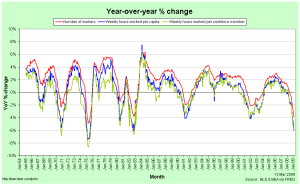
The Year-over-Year percentage changes in the number of employed workers, the weekly hours per capita and the weekly hours per workforce member continue to worsen.  The current recession is still not quite as bad as that in 1981/82 by this measure, but it’s so close as to make no difference.

Year-over-year changes in employment and hours worked

Just looking at year-over-year figures is a little deceptive, though, as it’s not just how far below the 0%-change line you fall that matters, but also how long you spend below it.  Notice, for example, that while the 2001 recession never saw catastrophically rapid falls in employment, it continued to decline for a remarkably long time.

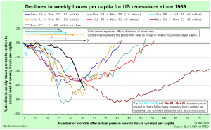
That’s why it’s useful to compare recessions in terms of their cumulative declines from peak:

Comparing US recessions relative to actual peaks in weekly hours worked per capitaA few points to note:

  • The figures are relative to the actual peak in weekly hours worked per capita, not to the official (NBER-determined) peak in economic activity.
  • I have shown the official recession durations (solid arrows) and the actual periods of declining weekly hours worked per capita (dotted lines) at the top.
  • The 1980 and 2001 recessions were odd in that weekly hours worked per capita never fully recovered before the next recession started.

The fact that the current recession isn’t yet quite as bad as the 1981/82 recession is a little clearer here.  The 1973-75 recession stands out as being worse than the current one and the 2001 recession was clearly the worst of all.

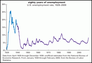
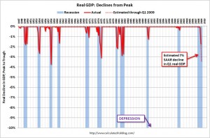
There’s also some question over the US is actually in a depression rather than just a recession.  The short answer is no, or at least not yet.  There is no official definition of a depression, but a cumulative decline of 10% in real GDP is often bandied around as a good rule of thumb.  Here are two diagrams that illustrate just how much worse things would need to be before the US was really in a depression …

First, from The Liscio Report, we have an estimated unemployment rate time-series that includes the Great Depression:

Historic Unemployment Rates in the USA

Second, from Calculated Risk, we have a time-series of cumulative declines in real gdp since World War II:

Cumulative declines in real GDP (USA)

Remember that we’d need to fall to -10% to hit the common definition of a depression.

More people have jobs AND the unemployment rate is higher

This is another one for my students in EC102.

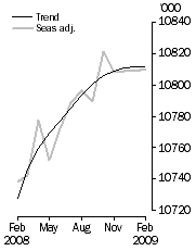
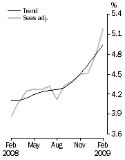
Via the always-worth-reading Peter Martin, I notice that the Australian Bureau of Statistics February release of Labour Force figures contains something interesting:  The number of people with jobs increased, but the unemployment rate still went up.  Here’s the release from the ABS:

Employed Persons Unemployment Rate
Australia Feb 2009 Employment Australia Feb 2009 Unemployment Rate

FEBRUARY KEY POINTS

TREND ESTIMATES (MONTHLY CHANGE)

  • EMPLOYMENT increased to 10,811,700
  • UNEMPLOYMENT increased to 561,100
  • UNEMPLOYMENT RATE increased to 4.9%
  • PARTICIPATION RATE increased to 65.4%

SEASONALLY ADJUSTED ESTIMATES (MONTHLY CHANGE)

EMPLOYMENT

  • increased by 1,800 to 10,810,400. Full-time employment decreased by 53,800 to 7,664,200 and part-time employment increased by 55,600 to 3,146,200.

UNEMPLOYMENT

  • increased by 47,100 to 590,500. The number of persons looking for full-time work increased by 44,400 to 426,000 and the number of persons looking for part-time work increased by 2,600 to 164,500.

UNEMPLOYMENT RATE

  • increased by 0.4 percentage points to 5.2%. The male unemployment rate increased by 0.3 percentage points to 5.1%, and the female unemployment rate increased by 0.5 percentage points to 5.3%.

PARTICIPATION RATE

  • increased by 0.2 percentage points to 65.5%.

The proximate reason is that more people want a job now than did in January.  The unemployment rate isn’t calculated using the total population, but instead uses the Labour Force, which is everybody who has a job (Employed) plus everybody who wants a job and is looking for one (Unemployed).

$$!u=\frac{U}{E+U}$$

Employment increased by 1,800, but unemployment increased by 47,100, so the unemployment rate ($$u$$) still went up.

Peter Martin also offered a suggestion on why this happened:

We’ve lost a lot of wealth and we’re worried. So those of us who weren’t looking for work are piling in.

I generally agree, but my guess would go further. Notice two things:

  • Part-time jobs went up by 55,600 and full-time jobs fell by 53,800 (the difference is the 1,800 increase in total employment).
  • The number of people looking for part-time jobs went up by only 2,600 and the number of people looking for full-time jobs rose by 44,400 (yes, I realise that there’s 100 missing – I guess the ABS has a typo somewhere).

There are plenty of other explanations, but I think that by and large, the new entrants to the Labour Force only wanted part-time work and found it pretty-much straight away – these are households that were single-income, but have moved to two-incomes out of the concern that Peter highlights.  On the other hand, I suspect that the people that lost full-time jobs have generally remained in the unemployment pool (some will have given up entirely, perhaps calling it retirement).

The aggregate result is that the economy had a shift away from full-time and towards part-time work, although the people losing the full-time jobs are not the ones getting the new part-time work.

Article Summary: Economics and Identity

You can access the published paper here and the unpublished technical appendices here.  The authors are George Akerlof [Ideas, Berkeley] and Rachel Kranton [Duke University].  The full reference is:

Akerlof, George A. and Kranton, Rachel E. “Economics and Identity.” Quarterly Journal of Economics, 2000, 115(3), pp. 715-53.

The abstract:

This paper considers how identity, a person’s sense of self, affects economic outcomes.We incorporate the psychology and sociology of identity into an economic model of behavior. In the utility function we propose, identity is associated with different social categories and how people in these categories should behave. We then construct a simple game-theoretic model showing how identity can affect individual interactions.The paper adapts these models to gender discrimination in the workplace, the economics of poverty and social exclusion, and the household division of labor. In each case, the inclusion of identity substantively changes conclusions of previous economic analysis.

I’m surprised that this paper was published in such a highly ranked economics journal.  Not because of a lack of quality in the paper, but because of it’s topic.  It reads like a sociology or psychology paper.  99% of the mathematics were banished to the unpublished appendices, while what made it in were the justifications by “real world” examples.  The summary is below the fold … Continue reading “Article Summary: Economics and Identity”

Is economics looking at itself?

Patricia Cowen recently wrote a piece for the New York Times:  “Ivory Tower Unswayed by Crashing Economy

The article contains precisely what you might expect from a title like that.  This snippet gives you the idea:

The financial crash happened very quickly while “things in academia change very, very slowly,” said David Card, a leading labor economist at the University of California, Berkeley. During the 1960s, he recalled, nearly all economists believed in what was known as the Phillips curve, which posited that unemployment and inflation were like the two ends of a seesaw: as one went up, the other went down. Then in the 1970s stagflation — high unemployment and high inflation — hit. But it took 10 years before academia let go of the Phillips curve.

James K. Galbraith, an economist at the Lyndon B. Johnson School of Public Affairs at the University of Texas, who has frequently been at odds with free marketers, said, “I don’t detect any change at all.” Academic economists are “like an ostrich with its head in the sand.”

“It’s business as usual,” he said. “I’m not conscious that there is a fundamental re-examination going on in journals.”

Unquestioning loyalty to a particular idea is what Robert J. Shiller, an economist at Yale, says is the reason the profession failed to foresee the financial collapse. He blames “groupthink,” the tendency to agree with the consensus. People don’t deviate from the conventional wisdom for fear they won’t be taken seriously, Mr. Shiller maintains. Wander too far and you find yourself on the fringe. The pattern is self-replicating. Graduate students who stray too far from the dominant theory and methods seriously reduce their chances of getting an academic job.

My reaction is to say “Yes.  And No.”  Here, for example, is a small list of prominent economists thinking about economics (the position is that author’s ranking according to ideas.repec.org):

There are plenty more. The point is that there is internal reflection occurring in economics, it’s just not at the level of the journals.  That’s for a simple enough reason – there is an average two-year lead time for getting an article in a journal.  You can pretty safely bet a dollar that the American Economic Review is planning a special on questioning the direction and methodology of economics.  Since it takes so long to get anything into journals, the discussion, where it is being made public at all, is occurring on the internet.  This is a reason to love blogs.

Another important point is that we are mostly talking about macroeconomics.  As I’ve mentioned previously, I pretty firmly believe that if you were to stop an average person on the street – hell, even an educated and well-read person – to ask them what economics is, they’d supply a list of topics that encompass Macroeconomics and Finance.

The swathes of stuff on microeconomics – contract theory, auction theory, all the stuff on game theory, behavioural economics – and all the stuff in development (90% of development economics for the last 10 years has been applied micro), not to mention the work in econometrics; none of that would get a mention.  The closest that the person on the street might get to recognising it would be to remember hearing about (or possibly reading) Freakonomics a couple of years ago.

Evil

Evil, I say:

Dozens of specially trained agents work on the third floor of DCM Services here, calling up the dear departed’s next of kin and kindly asking if they want to settle the balance on a credit card or bank loan, or perhaps make that final utility bill or cellphone payment.

The people on the other end of the line often have no legal obligation to assume the debt of a spouse, sibling or parent. But they take responsibility for it anyway.

Evil.

How to value toxic assets (part 6)

Via Tyler Cowen, I am reminded (again) that I should really be reading Steve Waldman more often.  Like, all the time.  After reading John Hempton’s piece that I highlighted last time, Waldman writes, as an afterthought:

There’s another way to generate price transparency and liquidity for all the alphabet soup assets buried on bank balance sheets that would require no government lending or taxpayer risk-taking at all. Take all the ABS and CDOs and whatchamahaveyous, divvy all tranches into $100 par value claims, put all extant information about the securities on a website, give ’em a ticker symbol, and put ’em on an exchange. I know it’s out of fashion in a world ruined by hedge funds and 401-Ks and the unbearable orthodoxy of index investing. But I have a great deal of respect for that much maligned and nearly extinct species, the individual investor actively managing her own account. Individual investors screw up, but they are never too big to fail. When things go wrong, they take their lumps and move along. And despite everything the professionals tell you, a lot of smart and interested amateurs could build portfolios that match or beat the managers upon whose conflicted hands they have been persuaded to rely. Nothing generates a market price like a sea of independent minds making thousands of small trades, back and forth and back and forth.

I don’t really expect anybody to believe me, but I’ve been thinking something similar.

CDOs, CDOs-squared and all the rest are derrivatives that are traded over the counter; that is, they are traded entirely privately.  If bank B sells some to hedge fund Y, nobody else finds out any details of the trade or even that the trade took place.  The closest we come is that when bank B announces their quarterly accounts, we might realise that they off-loaded some assets.

On the more popularly known stock and bond markets, buyers publicly post their “bid” prices and sellers post their “ask” prices. When the prices meet, a trade occurs.[*1] Most details of the trade are then made public – the price(s), the volume, the particular details of the asset (ordinary shares in XXX, 2-year senior notes from XXX with an expiry of xx/xx/xxxx, etc) – everything except the identity of the buyer and seller. Those details then provide some information to everybody watching on how the buyer and seller value the asset. Other market players can then combine that with their own private valuations and update their own bid or ask prices accordingly. In short, the market aggregates information. [*2]

When assets are traded over the counter (OTC), each participant can only operate on their private valuation. There is no way for the market to aggregate information in that situation. Individual banks might still partially aggregate information by making a lot of trades with a lot of other institutions, since each time they trade they discover a bound on the valuation of the other party (an upper bound when you’re buying and the other party is selling, a lower bound when you’re selling and they’re buying).

To me, this is a huge failure of regulation. A market where information is not publicly and freely available is an inefficient market, and worse, one that expressly creates an incentive for market participants to confuse, conflate, bamboozle and then exploit the ignorant. Information is a true public good.

On that basis, here is my idea:

Introduce new regulation that every financial institution that wants to get support from the government must anonymously publish all details of every trade that they’re party to. The asset type, the quantity, the price, any time options on the deal, everything except the identity of the parties involved. Furthermore, the regulation would be retroactive for X months (say, two years, so that we get data that predates the crisis).  On top of that, the regulation would require that every future trade from everyone (whether they were receiving government assistance or not) would be subject to the same requirementes.  Then everything acts pretty much like the stock and bond markets.

The latest edition of The Economist has an article effectively questioning whether this is such a good idea.

[T]ransparency and liquidity are close relatives. One enemy of liquidity is “asymmetric information”. To illustrate this, look at a variation of the “Market for Lemons” identified by George Akerlof, a Nobel-prize-winning economist, in 1970. Suppose that a wine connoisseur and Joe Sixpack are haggling over the price of the 1998 Château Pétrus, which Joe recently inherited from his rich uncle. If Joe and the connoisseur only know that it is a red wine, they may strike a deal. They are equally uninformed. If vintage, region and grape are disclosed, Joe, fearing he will be taken for a ride, may refuse to sell. In financial markets, similarly, there are sophisticated and unsophisticated investors, and unless they have symmetrical information, liquidity can dry up. Unfortunately transparency may reduce liquidity. Symmetry, not the amount of information, matters.

I’m completely okay with this. Symmetric access to information and symmetric understanding of that information is the ideal. From the first paragraph and then the last paragraph :

… Not long ago the cheerleaders of opacity were the loudest. Without privacy, they argued, financial entrepreneurs would be unable to capture the full value of their trading strategies and other ingenious intellectual property. Forcing them to disclose information would impair their incentive to uncover and correct market inefficiencies, to the detriment of all …

Still, for all its difficulties, transparency is usually better than the alternative. The opaque innovations of the recent past, rather than eliminating market inefficiencies, unintentionally created systemic risks. The important point is that financial markets are not created equal: they may require different levels of disclosure. Liquidity in the stockmarket, for example, thrives on differences of opinion about the value of a firm; information fuels the debate. The money markets rely more on trust than transparency because transactions are so quick that there is little time to assess information. The problem with hedge funds is that a lack of information hinders outsiders’ ability to measure their contribution to systemic risk. A possible solution would be to impose delayed disclosure, which would allow the funds to profit from their strategies, provide data for experts to sift through, and allay fears about the legality of their activities. Transparency, like sunlight, needs to be looked at carefully.

This strikes me as being around the wrong way.  Money markets don’t rely on trust because their transactions are so fast; their transactions are so fast because they’re built on trust.  The scale of the crisis can be blamed, in no small measure, because of the breakdown in that trust.

I also do not buy the idea of opacity begetting market efficiency.  It makes no sense.  The only way that information disclosure can remove the incentive to “uncover and correct” inefficiencies in the market is if by making the information public you reduce the inefficiency.  I’m not suggesting that we force market participants to reveal what they discover before they get the chance to act on it.  I’m only suggesting that the details of their action should be public.

[*1] Okay, it’s not exactly like that, but it’s close enough.

[*2] Note that information aggregation does not necessarily imply that the Efficient Market Hypothesis (EMH), but the EMH requires information aggregation to work.

Other posts in this series:  1, 2, 3, 4, 5, [6].